library(rio)
library(tidyverse)
library(TraMineR)
library(seqHMM)
library(WeightedCluster) 13 Multi-channel sequence analysis in educational research: An introduction and tutorial with R
Abstract
This chapter introduces multi-channel sequence analysis, a novel method that examines two or more synchronised sequences. While this approach is relatively new in social sciences, its relevance to educational research is growing as researchers gain access to diverse multimodal temporal data. Throughout this chapter, we describe multi-channel sequence analysis in detail, with an emphasis on how to detect patterns within the sequences, i.e., clusters —or trajectories— of multi-channel sequences that share similar temporal evolutions (or similar trajectories). To illustrate this method we present a step-by-step tutorial in R that analyses students’ sequences of online engagement and academic achievement, exploring their longitudinal association. We cover two approaches for clustering multi-channel sequences: one based on using distance-based algorithms, and the other employing mixture hidden Markov models inspired by recent research.
13.1 Introduction
Learning is a dynamic phenomenon which follows the unidirectional forward law of time; that is, learning occurs sequentially in a time-ordered manner [1, 2]. Throughout this book, we have devoted several chapters to sequence analysis of learner-related data, due to its increasingly central role in learning analytics and education research as a whole. First, in Chapter 10 [3], we presented an introduction to sequence analysis and a discussion on the relevance of this method. Subsequently, in Chapter 11 [4], we studied how to build sequences from multiple variables and analyse more complex aspects of sequences. Both Chapter 10 and Chapter 11 also deal with clustering sequences into trajectories which undergo a similar evolution using distance-based methods. Then, in Chapter 12 [5], we learned how to cluster sequential data using Markov models. Though Chapter 12 [5] touched briefly on simultaneous analysis of multi-channel sequences —albeit only from the Markovian point of view— we present the multi-channel perspective in greater detail here.
In this new chapter, we cover multi-channel sequence analysis, which deals with the analysis of two or more synchronised sequences, in greater detail. An example in educational research would be the analysis of the simultaneous unfolding of motivation, achievement, and engament sequences. Multi-channel sequence analysis is a rather novel method in social sciences [6–9] and its applications within educational research in general remain scarce. The increasing availability of student multimodal temporal data makes multi-channel sequence analysis a relevant and timely method to tackle the challenges that these new data bring.
Throughout this chapter, we describe multi-channel sequence analysis in detail, with an emphasis on how to detect patterns within the sequences, i.e., clusters —or trajectories— of multi-channel sequences that share similar temporal evolutions (or similar trajectories). We illustrate the method with a case study in which we examine students’ sequences of online engagement and academic achievement, where we analyse the longitudinal association between both constructs simultaneously. Here, we outline two perspectives on clustering multi-channel sequences and present both in the tutorial. The first approach uses distance-based clustering algorithms, very much in the spirit of the single-channel cluster analysis described in Chapter 10. We describe some limitations of this framework and then principally focus on a more efficient approach to identifying distinct trajectories using mixture hidden Markov models. We also show how covariates can be incorporated to make the Markovian framework even more powerful. This main analysis is inspired by the recently published paper by [10]. In the next section, we provide a description of the multi-channel sequence analysis framework. We follow with a review of the existing literature in learning analytics that has relied on multi-channel sequence analysis. Next, we include a step-by-step tutorial on how to implement multi-channel sequence analysis with R, with particular attention paid to clustering via distance-based algorithms and mixture hidden Markov models. Finally, we conclude with a brief discussion and provide recommendations for further reading.
13.2 Multi-channel sequence analysis
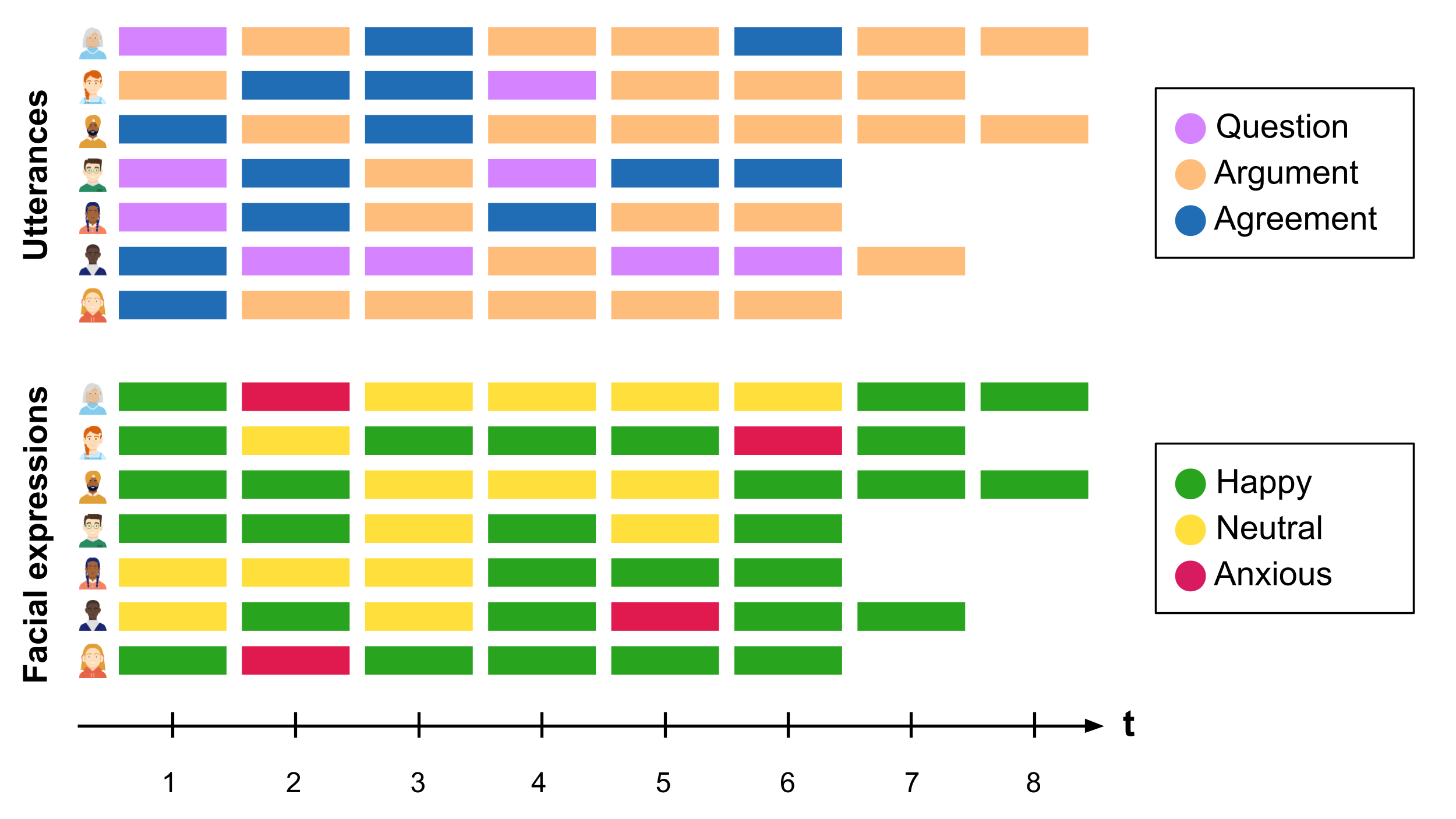
Multi-channel sequence analysis refers to the process of analysing sequential data that consists of multiple parallel channels or streams of (categorical) information. Each channel provides a different perspective or type of information. The goal of multi-channel sequence analysis is to jointly explore the dependencies and temporal interactions between the different channels and extract meaningful insights that may not be evident when considering each channel in isolation. The sources of information can be of very varied nature. For example, using video data of students working on a collaborative task, we could code students’ spoken utterances in one channel, and their facial expressions in another channel throughout the whole session (see Figure 13.1). In this way, we could analyse how students’ expressions relate to what they are saying. Multi-channel sequence analysis often follows the following steps:
13.2.1 Step 1: Building the channel sequences
Just like in regular sequence analysis (see Chapter 10 [3]), the first step in multi-channel sequence analysis is to construct the sequences which constitute the different channels. A sequence is an ordered list of categorical elements (i.e., events, states or categories). These elements are discrete (as opposed to numerical values such as grades) and are ordered chronologically. In a sequence, time is not a continuum but a succession of discrete timepoints. These timepoints can be generated by sampling (e.g., each 30 seconds constitutes a new timepoint) or can emerge from an existing time scheme (e.g., each new lesson in a course is a new timepoint). In multi-channel sequence analysis, it is very important that all channels (i.e., parallel sequences) follow the same time scheme so they can be synchronised. As well as time points being aligned in this fashion, it is also typically assumed that the sequence length for each observation matches across channels (although some of the methods used can also deal with partially missing information). The elements of each sequence —typically referred to as the alphabet, which is unique for each channel— can be predefined events or categories from the beginning (e.g., utterances or facial expressions) or, in cases where we are dealing with numerical variables (e.g., heart rate or grades), we can convert them into a state or category by dividing the numerical variable into levels (e.g., tertiles, quartiles) or using clustering techniques. This way, we can focus on sharp changes in numerical variables and conceal small, probably insignificant changes. As Winne puts it [11], “reliability can sometimes be improved by tuning grain size of data so it is neither too coarse, masking variance within bins, nor too fine-grained, inviting distinctions that cannot be made reliably”. Once we have our channels represented as sequences of ordered elements that follow the same time scheme, we can use the steps learned in the introductory sequence analysis chapter to construct the sequences.
13.2.2 Step 2: Visualising the multi-channel sequence
When we have built the sequences corresponding to all of the channels, we can visualise the data. Visualising multi-channel sequence data is not a straightforward task, and we need to decide whether we want to present each channel separately or extend the alphabet to show a plot of combined states—or sometimes even both. The extended alphabet approach —in which the states are the combination of the states of all the channels— helps us understand the structure of the data and the typical combinations and evolution of the combined states from all of the channels. It usually works well when (1) the extended alphabet is moderate in size, (2) when there are no state combinations that are very rare, and (3) when the states are either fully observed or missing in all channels at the same time. The extended alphabet is likely to be of moderate size when there are at most 2–3 channels with a small alphabet in each, or if some combinations are not present in the data. Rare state combinations are typically impractical both when visualizing and analyzing the data—especially if there are many rare combinations or if the data are very sensitive in nature. Finally, if there are partially missing observations, i.e., observations that at some specific time point are missing from some of the channels but not all, we would need to deal with each combination of missing and observed states separately, which further extends the alphabet. If one or more of the three conditions are not met, it is often preferable to resort to presenting each channel separately or using visualization techniques that summarise information (e.g., sequence distribution plots).
Continuing with the previous example, the possible states in the extended alphabet would be all the combinations between the alphabet of the utterances channel (Question-Argument-Agreement) and the alphabet of the facial expressions channel (Happy-Neutral-Anxious). In Figure 13.2, we can see that the first student starts by ‘Question/Happy’, then goes to ‘Argument/Anxious’ and so on.

13.2.3 Step 3: Finding patterns (clusters or trajectories)
Patterns may exist in all types of sequences and, in fact, in all types of data. Discovering such patterns, variations, or groups of patterns is a central theme in analytics. In sequence analysis, similar patterns reflect common temporal pathways where the data share a similar temporal course. This could be a group of students, a typical succession of behavior, or a sequence of interactions. As such, the last typical step in the analysis is to find such patterns. Since these patterns are otherwise latent or unobservable, we need a clustering algorithm that unveils such hidden patterns. There are different possibilities to cluster multi-channel sequence data, of which two are described below: extensions to traditional distance-based clustering approaches widely used in single-channel analyses and Markovian models. The two approaches are then further distinguished in Section Section 13.2.4, with regard to the ability of the Markovian approach to directly accommodate covariates.
13.2.3.1 Traditional sequence analysis extensions
Broadly speaking, the first paradigm involves extending techniques commonly adopted in single-channel analyses to the multi-channel domain, by suitably summarising the information arising from all constituent channels. Within this first framework, two different approaches have been proposed.
The first consists of flattening the multi-channel data by combining the states (such as in the example in Figure 13.2) and treating the sequence as a single channel with an extended alphabet. Typically, one would then compute dissimilarities using this extended alphabet, most commonly using Optimal Matching (OM). However, this approach is not limited to distance-based clustering [12]; any of the methods, distance-based or otherwise, that we have seen in the previous chapters related to sequence analysis can be used to cluster sequences represented in this way (e.g., agglomerative hierarchical clustering using OM, or hidden Markov models). While this seems like an easier choice, the models tend to become too complex —in the sense of requiring a larger number of clusters and/or hidden states in order to adequately characterise the data— when the number of channels or numbers of per-channel states increase. Moreover, for even a moderate number of channels and/or moderate numbers of states per-channel, the size of the combined alphabet can become unwieldy. Indeed, using this approach in conjunction with OM has been criticised because of the difficulty of specifying appropriate substitution costs for such large combined alphabets [13]. As a reminder, the substitution cost refers to the penalty associated with replacing one element of a sequence with another one; these dissimilarites between all pairs of states are then used to calculate all pairwise distances between whole sequences, which are treated as the input to distance-based clustering algorithms (see Chapter 10 [3]).
The second, more common approach is explicitly distance-based and relies on an extension of the OM metric itself, by using a set of overall multi-channel costs derived from channel-specific costs, to calculate a pairwise dissimilarity matrix. The method relies on computing substitution costs for each constituent channel, combining the channels into a new multi-channel sequence object, and deriving an overall substitution cost matrix for the multi-channel object by adding (or averaging) the appropriate substitution costs across channels for a particular multi-state change, typically with equal weight given to each channel [14]. For instance, if the cost associated with substituting the states ‘Question’ and ‘Agreement’ in the utterances channel in Figure 13.1 is \(0.6\) and the cost of substituting ‘Happy’ and ‘Neutral’ in the facial expressions channel is \(1.2\), the cost associated with substitutions of ‘Question/Neutral’ for ‘Question/Happy’ and ‘Question/Neutral’ for ‘Agreement/Happy’ in Figure 13.2 would be \(1.2\) and \(1.8\), respectively. From such multi-channel costs, a pairwise multi-channel dissimilarity matrix can be obtained and all subsequent steps of the clustering analysis can proceed as per Chapter 10 thereafter.
That being said, adopting the extended OM approach rather than the extended alphabet approach does not resolve all limitations of the distance-based clustering paradigm. As Saqr et al. [15] noted, large sequences are hard to cluster using standard methods such as hierarchical clustering, which is memory inefficient and hard to parallelise or scale [16, 17]. Furthermore, distance-based clustering methods are limited by the theoretical maximum dimension of a matrix in R which is 2,147,483,647, corresponding to a maximum of 46,430 sequences. Using weights can fix the memory issue if the number of unique sequences remains below the threshold [18]. However, the more states (and combinations of states), the more unique the sequences tend to be, so the memory issue is even more typical with multi-channel sequence data. In such a case, Markovian methods may be the solution. Moreover, the particular choice of distance-based clustering algorithm must be chosen with care, and as ever the user must pre-specify the number of clusters, thereby often necessitating the evaluation of several computing solutions with different numbers of clusters, different hierarchical clustering linkage criteria, or different distance-based clustering algorithms entirely.
13.2.4 Step 4: Relating clusters to covariates
As we have seen, there are, broadly speaking, two conflicting perspectives on clustering in the sequence analysis community; algorithmic, distance-based clustering on the one hand, and model-based clustering on the other. Distance-based clustering of multi-channel sequences has already been described above, but it is useful to acknowledge that mixture Markov models and mixture hidden Markov models are precisely examples of model-based clustering methods. Moreover, seqHMM and the methods it implements are unique in offering a model-based approach to clustering multi-channel sequences. A key advantage of the model-based clustering framework is that it can easily be extended to directly account for information available in the form of covariates, as part of the underlying probabilistic model. Though the recently introduced mixture of exponential-distance models framework [22] attempts to reconcile the distance-based and model-based cultures in sequence analysis, while allowing for the direct incorporation of covariates, it is not based on Markovian principles, and most importantly can currently only accommodate single-channel sequences.
Otherwise, however, distance-based approaches typically cannot accommodate covariates, except as part of a post-hoc step whereby, typically, covariates are used as explanatory variables in a post-hoc multinomial regression with the cluster memberships used as the response (or as independent variables in linear or non-linear regression models). This is questionable as substituting a categorical variable indicating cluster membership disregards the heterogeneity within clusters and is clearly only sensible when the clusters are sufficiently homogeneous [23, 24]. It is often more desirable to incorporate covariates directly, i.e. to cluster sequences and relate the clusters to the covariates simultaneously. This represents an important distinction between the two approaches outlined above; this step does not apply to distance-based clustering approaches and is a crucial advantage of the Markovian approach which makes MHMMs even more powerful tools for clustering multi-channel sequences.
In theory, MHMMs can include covariates to explain the initial, transition, and/or emission probabilities. A natural use-case would be to allow subject-specific and possibly time-varying transition and emission probabilities (in the case of time-varying covariates). For example, if we think that transitioning from low to high achievement gets harder as the students get older we may add time as an explanatory variable to the model, allowing the probability of transitioning from low to high achievement to diminish in time. However, at the time of writing this chapter, these extensions are not supported in seqHMM (this may change in the future). Instead, the seqHMM package used in the examples supports time-constant covariates only. Specifically, the manner in which covariates are accommodated is similar in spirit to the aforementioned mixture of exponential-distance models framework and latent class regression [25], in that covariates are used for predicting cluster memberships for each observed sequence. Adding covariates to the model thus helps to both explain and influence the probabilities that each individual has of belonging to each cluster. By incorporating covariates in this way, we could, for example, find that being in a high-achievement cluster is predicted by gender, previous grades, or family background
In the terminology of mixtures of experts modelling, this approach corresponds to a so-called “gating network mixture of experts model”, whereby the distribution of the sequences depends on the latent cluster membership variable, which in turn depends on the covariates, while the sequences are independent of the covariates, conditional on the latent cluster membership variable (see [26] and [22] for examples). This, rather than having covariates affect the component distributions, is particularly appealing, as the interpretation of state-specific parameters is the same as it would be under a model without covariates. However, it is worth noting that the covariates do not merely explain the uncovered clusters; as part of the model, they drive the formation of the clusters. In other words, an otherwise identical model without dependence on covariates may uncover different groupings with different probabilities. However, this can be easily overcome by treating the selection of the most relevant subset of covariates as an issue of model selection via the BIC or other criteria and taking the number of clusters/states, set of initial probabilities, and set of covariates which jointly optimise the chosen criterion. The incorporation of covariates in MHMMs and related practical issues are also illustrated in the case study on the longitudinal association of engagement and achievement which follows.
13.3 Review of the literature
The use of multi-channel sequence analysis in learning analytics has so far been scarce. Most of the few studies that implemented this method used it to combine multiple modalities of data such as coded video data [27, 28], electrodermal activity [27, 28], clickstream/logged data [10, 29, 30], and assessment/achievement data [10, 30, 31]. The data were converted into different sequence channels using a variety of methods. For example, [27] manually coded video interactions as positive/negative/mixed to represent the emotional valence of individual interaction, and used a pre-defined threshold to discern between high and low arousal from electrodermal activity data. In the work by [30], two sequence channels were built from students’ daily tactics using the learning management system and an automated assessment tool for programming assignments respectively. The learning tactics were identified through hierarchical clustering of students’ trace log data in each environment. Similarly [10], created an engagement channel for each course in a study program based on students’ engagement states derived from the learning management system data, and an achievement state based on their grade tertiles. Another study [29] had five separate channels: the first channel represented the interactive dimension built from the social interactions through peer communications and online behaviours; the second channel represented the cognitive dimension constructed from students’ knowledge contributions at the superficial, medium, and deep levels; the third channel represented the regulative dimension which represented students’ regulation of their collaborative processes, including task understanding, goal setting and planning, as well as monitoring and reflection; the fourth channel represented the behavioural dimension which analysed students’ online behaviours, including resource management, concept mapping and observation, and the fifth channel represented the socio-emotional dimension, which included active listening and respect, encouraging participation and inclusion, as well as fostering cohesion.
A common step in the existing works is the use of clustering techniques to detect unobserved patterns within the multi-channel sequences. Articles have relied on hidden Markov models to identify hidden states in the data. For instance, [30] found three hidden states consisting of learning strategies which combine the use of the learning management system and an automated assessment tool: an instruction-oriented strategy where students consume learning resources to learn how to code; an independent coding strategy where students relied on their knowledge or used the learning resources available to complete the assignments, and a dependent coding strategy where students mostly relied on the help forums to complete their programming assignments. Most studies go one step further and identify distinct trajectories based on such hidden states. For example, [28] found four clusters of socio-emotional interaction episodes (positive, negative, occasional regulation, frequent regulation), which differed in terms of fluctuation of affective states and activated regulation of learning. The authors of [29] found three types of group collaborative patterns: behaviour-oriented, communication-behaviour-synergistic, and communication-oriented. To the knowledge of the authors, no article has relied on the distance-based approach (commonly used in single-channel sequence analysis) to cluster multi-channel sequences. However, this approach has been used in social sciences [9] as well as in other disciplines [e.g., 32].
13.4 Case study: the longitudinal association of engagement and achievement
To learn how to implement multi-channel sequence analysis we are going to practice with a real case study: we will investigate the longitudinal association between engagement and achievement across a study program using simulated data based on the study by [10]. We begin by creating a sequence for each of the channels (engagement and achievement) and then explore visualisations thereof. We then focus on clustering these data using the methods described above specifically tailored for multi-channel sequences, in order to present an empirical view of both the distance-based and Markovian perspectives. In doing so, we will first demonstrate how to construct a multi-channel pairwise OM dissimilarity matrix in order to adapt and apply the distance-based clustering approach of Chapter 10 to these data. Secondly, we will largely focus on using a mixture hidden Markov model to detect the longitudinal clusters of students that share a similar trajectory of engagement and achievement. Finally, we will demonstrate how to incorporate covariates under the model-based Markovian framework.
13.4.1 The packages
To accomplish our task, we will rely on several R packages We have use most of them throughout the book. Below is a brief summary of the packages required:
rio: A package for reading and saving data files with different extensions [33].seqHMM: A package designed for fitting hidden (latent) Markov models and mixture hidden Markov models for social sequence data and other categorical time series [21].tidyverse: A package that encompasses several basic packages for data manipulation and wrangling [34].TraMineR: As seen in the introductory sequence analysis chapter, this package helps us construct, analyse, and visualise sequences from time-ordered states or events [35].WeightedCluster: A package to cluster sequences and computing quality measures [18].
If you have not done so already, install the packages using the install.packages() command (e.g., install.packages("seqHMM")). We can then import them as follows:
13.4.2 The data
The data that we are going to use in this chapter is a synthetic dataset which contains the engagement states (Active, Average, or Disengaged) and achievement states (Achiever, Intermediate, or Low) for eight successive courses (each course is a timepoint). Each row contains an identifier for the student (UserID), an identifier for the course (CourseId), and the order (Sequence) in which the student took that course (1–8). For each course, a student has both an engagement state (Engagement) and an achievement state (Achievement). For example, a student can be 'Active' and 'Achiever' in the first course (Sequence = 1) they take, and 'Disengaged' and 'Low' achiever in the next. In addition, the dataset contains the final grade (0-100) and three time-constant covariates (they are the same for each student throughout all four courses): the previous grade (Prev_grade, 1-10), Attitude (0-20), and Gender (Male/Female). The dataset is described in more detail in the Data chapter of this book. We can import the data using the ìmport() command from rio:
URL <- "https://github.com/sonsoleslp/labook-data/raw/main/"
fileName <- "9_longitudinalEngagement/SequenceEngagementAchievement.xlsx"
df <- import(paste0(URL, fileName))
df
13.4.3 Creating the sequences
We are going to first construct and visualise each channel separately (engagement and achievement), and then study them in combination.
13.4.3.1 Engagement channel
To build the engagement channel, we need to construct a sequence of students’ engagement states throughout the eight courses. To do so, we need to first arrange our data by student (UserID) and course order (Sequence). Then, we pivot the data to a wide format, where the first column is the UserID and the rest of the columns are the engagement states at each of the courses (ordered from 1 to 8). For more details about this process, refer to the introductory sequence analysis chapter.
eng_seq_df <- df |> arrange(UserID, Sequence) |>
  pivot_wider(id_cols = "UserID", names_from = "Sequence", values_from = "Engagement")
Now we can use TraMineR to construct the sequence object and assign colours to it to represent each of the engagement states:
engagement_levels <- c("Active", "Average", "Disengaged")
colours <- c("#28a41f", "#FFDF3C", "#e01a4f")
eng_seq <- seqdef(eng_seq_df , 2:9, alphabet = engagement_levels, cpal = colours)
We can use the sequence distribution plot from TraMineR to visualise the distributions of the states at each time point (Figure 13.3 left), and the sequence index plot to visualise each student’s sequence of engagement states (Figure 13.3, right), here sorted according to the elements of the alphabet at the successive positions starting from the beginning of the sequences:
seqdplot(eng_seq, border = NA,  ncol = 3, legend.prop = 0.2)
seqIplot(eng_seq, border = NA,  ncol = 3, legend.prop = 0.2, sortv = "from.start")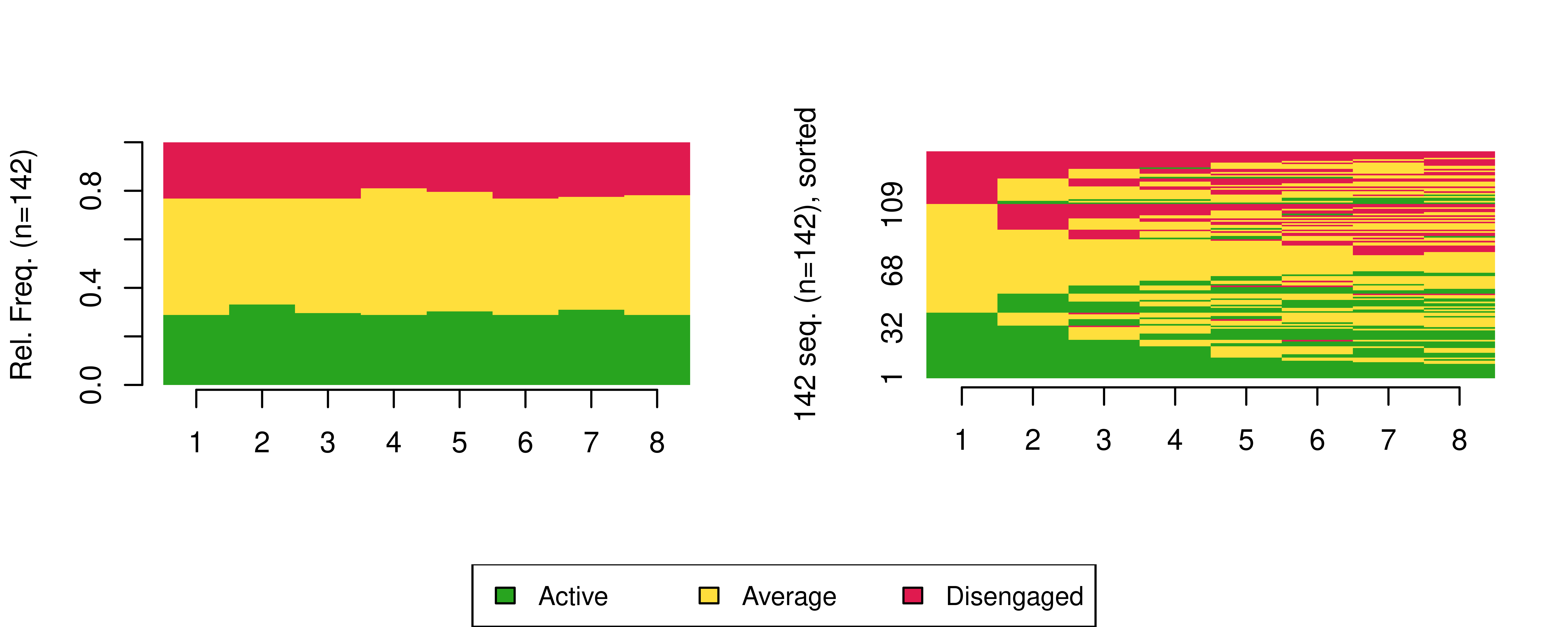
Please refer to Chapter 10 [3] for guidance on how to interpret sequence distribution and index plots.
13.4.3.2 Achievement channel
We follow a similar process to construct the achievement sequences. First we arrange the data by student and course order and then we convert the data into the wider format using —this time— the achievement states as the values.
ach_seq_df <- df |> arrange(UserID,Sequence) |>
  pivot_wider(id_cols = "UserID", names_from = "Sequence", values_from = "Achievement")
We use again TraMineR to construct the sequence object for achievement and we again provide a suitable, distinct colour scheme:
achievement_levels <- c("Low", "Intermediate", "Achiever")

coloursA <- c("#a5e3ff","#309bff","#3659bf")
ach_seq <- seqdef(ach_seq_df , 2:9, cpal = coloursA, alphabet = achievement_levels)
We may use the same visualisations to plot our achievement sequences in Figure 13.4:
seqdplot(ach_seq, border = NA,  ncol = 3, legend.prop = 0.2)
seqIplot(ach_seq, border = NA,  ncol = 3, legend.prop = 0.2, sortv = "from.start")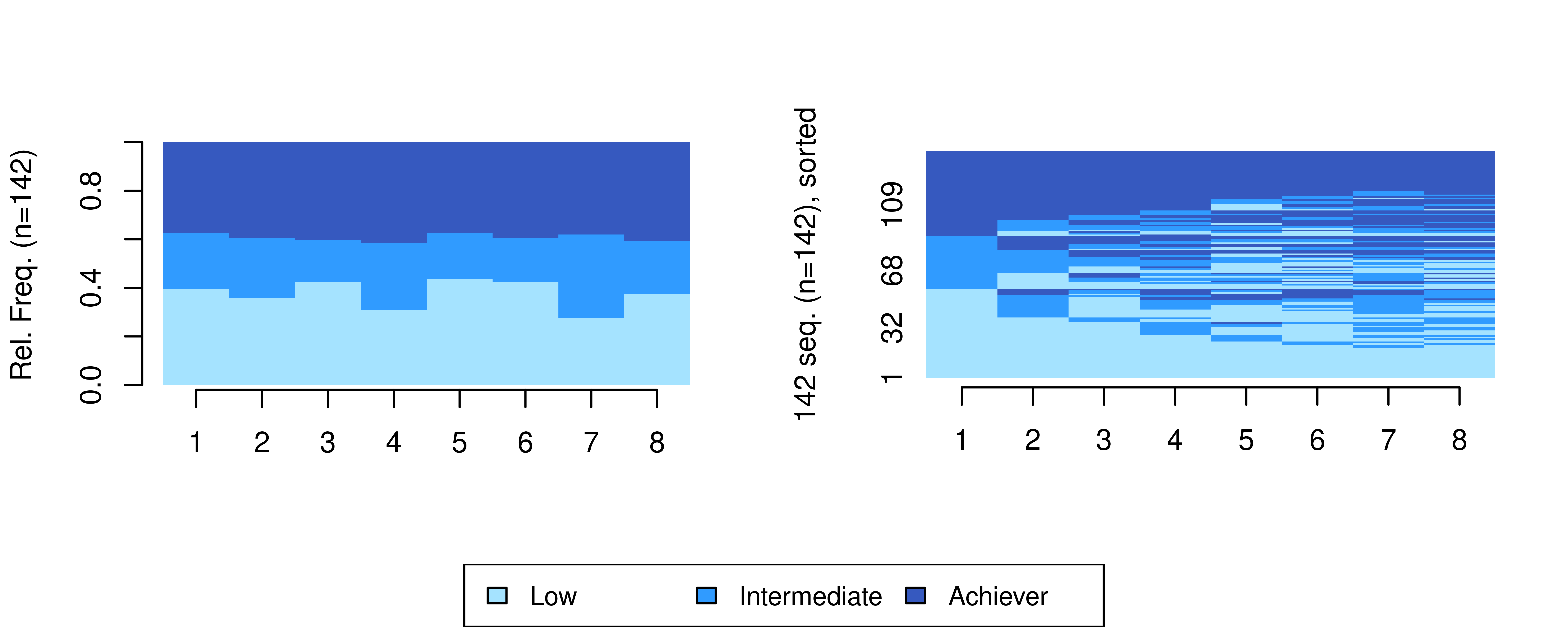
13.4.3.3 Visualising the multi-channel sequence
Now that we have both channels, we can use the mc_to_sc_data() function from seqHMM to convert the two channels of engagement and achievement sequences to a single channel with an extended alphabet. If we had additional channels, we would just add them to the list, after ach_seq.
multi_seq <- mc_to_sc_data(list(eng_seq, ach_seq))If we check the alphabet of the sequence data, we can see that it contains all combinations of engagement and achievement states.
alphabet(multi_seq)[1] "Active/Achiever" "Active/Intermediate"
[3] "Active/Low" "Average/Achiever"
[5] "Average/Intermediate" "Average/Low"
[7] "Disengaged/Achiever" "Disengaged/Intermediate"
[9] "Disengaged/Low" We now need to provide an appropriate colour scale to accommodate the extended alphabet. The colour scale we define below uses green colours to represent active students, blue colours represent averagely engaged students, and red colours represent disengaged students, whereas the intensity of the colour represents the achievement level: darker colours represent higher achievement, and lighter colours represent low achievement.
coloursM <-  c("#115a20","#24b744","#78FA94",
               "#3659bf","#309bff","#93d9ff",
               "#E01A1A","#EB8A8A","#F5BDBD")

cpal(multi_seq) <- coloursM
We can finally plot the sequence distribution and index plots for the multi-channel sequence (Figure 13.5). We can already hint that the students’ multi-channel sequences are quite heterogeneous. In the next steps, we will use two distinct clustering techniques to detect distinct combined trajectories of engagement and achievement, beginning with the distance-based paradigm and then the using the more sophisticated MHMM framework.
seqdplot(multi_seq, border = NA,  ncol = 3, legend.prop = 0.2)
seqIplot(multi_seq, border = NA,  ncol = 3, legend.prop = 0.2, sortv = "from.start")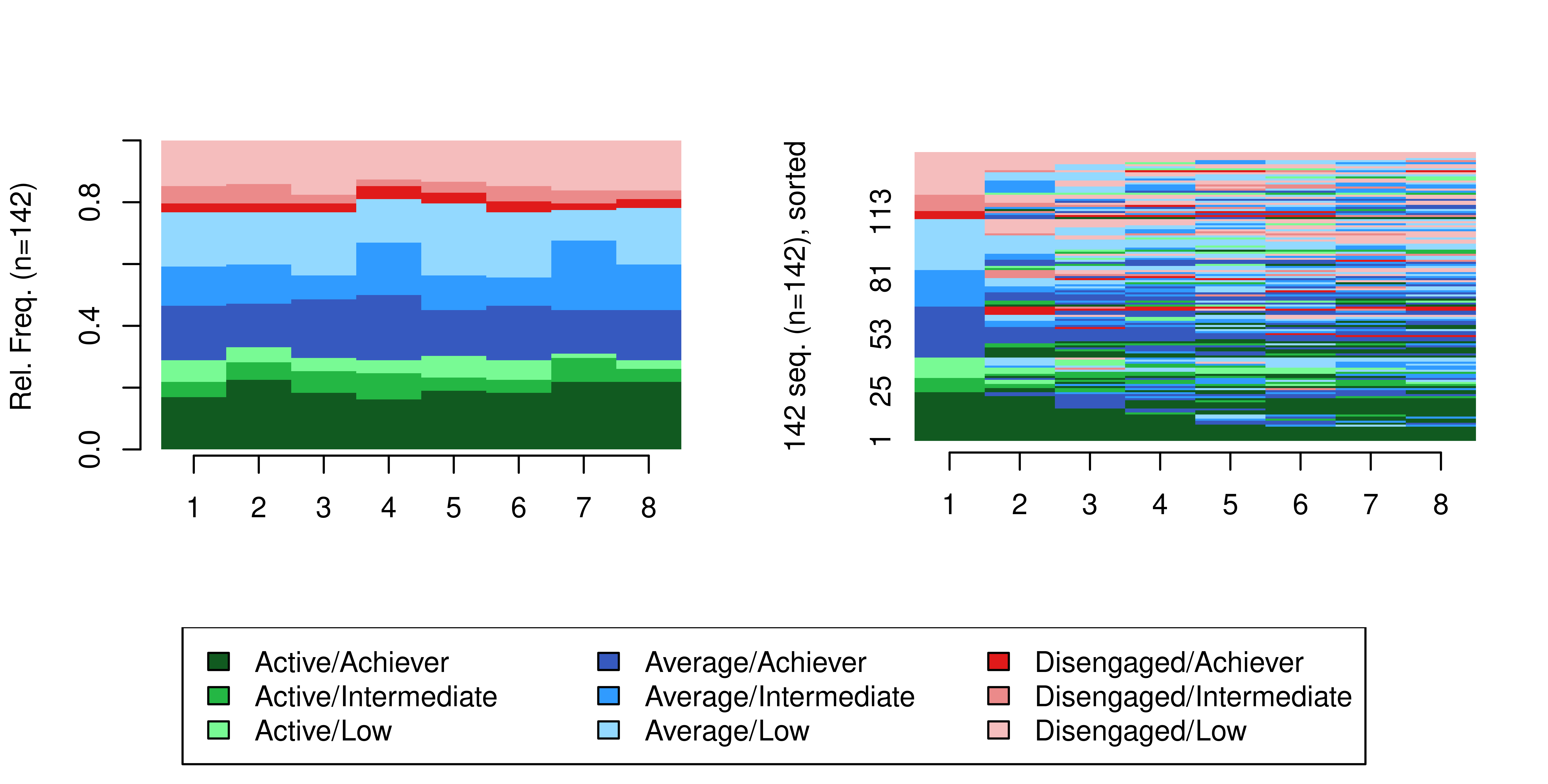
13.4.4 Clustering via multi-channel dissimilarities
We now describe how to construct a dissimilarity matrix for a combined multi-channel sequence object to use as input for distance-based clustering algorithms, using utilities provided in the TraMineR R package and relying on concepts described in Chapter 10. We begin by creating a list of substitution cost matrices for each of the engagement and achievement channels. For simplicity, we adopt the same method of calculating substitution costs for each channel, though this need not be the case. Here, we use the data-driven "TRATE" method, which relies on transition rates, as the method argument in both calls to seqsubm()}.In other scenarios, we might want to use a constant substitution cost (same cost for all substitutions) for one or some of the channels and, for example, manually specify the substitution cost matrix for the others.
sub_mats <- list(engagement = seqsubm(eng_seq, method = "TRATE"),
                 achievement = seqsubm(ach_seq, method = "TRATE"))
Subsequently, we invoke the function seqMD() to compute the multi-channel dissimilarities. This requires the constituent channels to be supplied as a list of sequence objects, along with the substitution cost matrices via the argument sm. The argument what = "diss" ensures that dissimilarities are returned, according to the OM method, with equal weights for each channel specified via the argument cweight.
channels <- list(engagement = eng_seq, achievement = ach_seq)

mc_dist <- seqMD(channels,
                 sm = sub_mats,
                 what = "diss",
                 method = "OM",
                 cweight = c(1, 1))
Thereafter, mc_dist can be used as input to any distance-based clustering algorithm. Though we are not limited to doing so, we follow Chapter 10 in applying hierarchical clustering with Ward’s criterion. However, we note that users of the distance-based paradigm are not limited to Ward’s criterion or hierarchical clustering itself either.
Clustered <- hclust(as.dist(mc_dist), method = "ward.D2")We then obtain the implied clusters by cutting the produced tree using the cutree() function, where the argument k indicates the desired number of clusters. We also create more descriptive labels for each cluster.
Cuts <- cutree(Clustered, k = 6)
Groups <- factor(Cuts, labels = paste("Cluster", 1:6))
It is worth noting that the Groups vector contains the clustering assignment for each student. This vector is a factor in the same order as the engagement and achievement sequences, and hence the same order as the data frames used to create the sequences. Hence, information about which student belongs to which cluster is readily accessible. Here, we show the assignments of the first 5 students only, for brevity.
head(Groups, 5) 1 2 3 4 5
Cluster 1 Cluster 2 Cluster 3 Cluster 4 Cluster 3
Levels: Cluster 1 Cluster 2 Cluster 3 Cluster 4 Cluster 5 Cluster 6Generally speaking, the resulting clusters for the chosen k value may not represent the best solution. In an ideal analysis, one would resort to one or more of the cluster quality measures given in Table 9 of Chapter 10 to inform the choice of an optimal k value. In doing so, we determined the chosen number of six clusters is optimal according to the average silhouette width (ASW) criterion (again, see Chapter 10). However, we omit repeating the details of these steps here for brevity and leave them as an exercise for the interested reader.
The obtained Groups can be used to produce visualisations of the clustering solution. We do so in two ways; first showing the combined multi-channel object with an extended alphabet (as per Figure 13.2) using the seqplot() function from TraMiner in Figure 13.6, and second using a stacked representation of both constituent channels using the ssp() and gridplot() functions from seqHMM in Figure 13.7. State distribution plots per cluster are depicted in each case.
seqplot(multi_seq, type = "d", group = Groups,
         ncol = 3, legend.prop = 0.1, border = NA)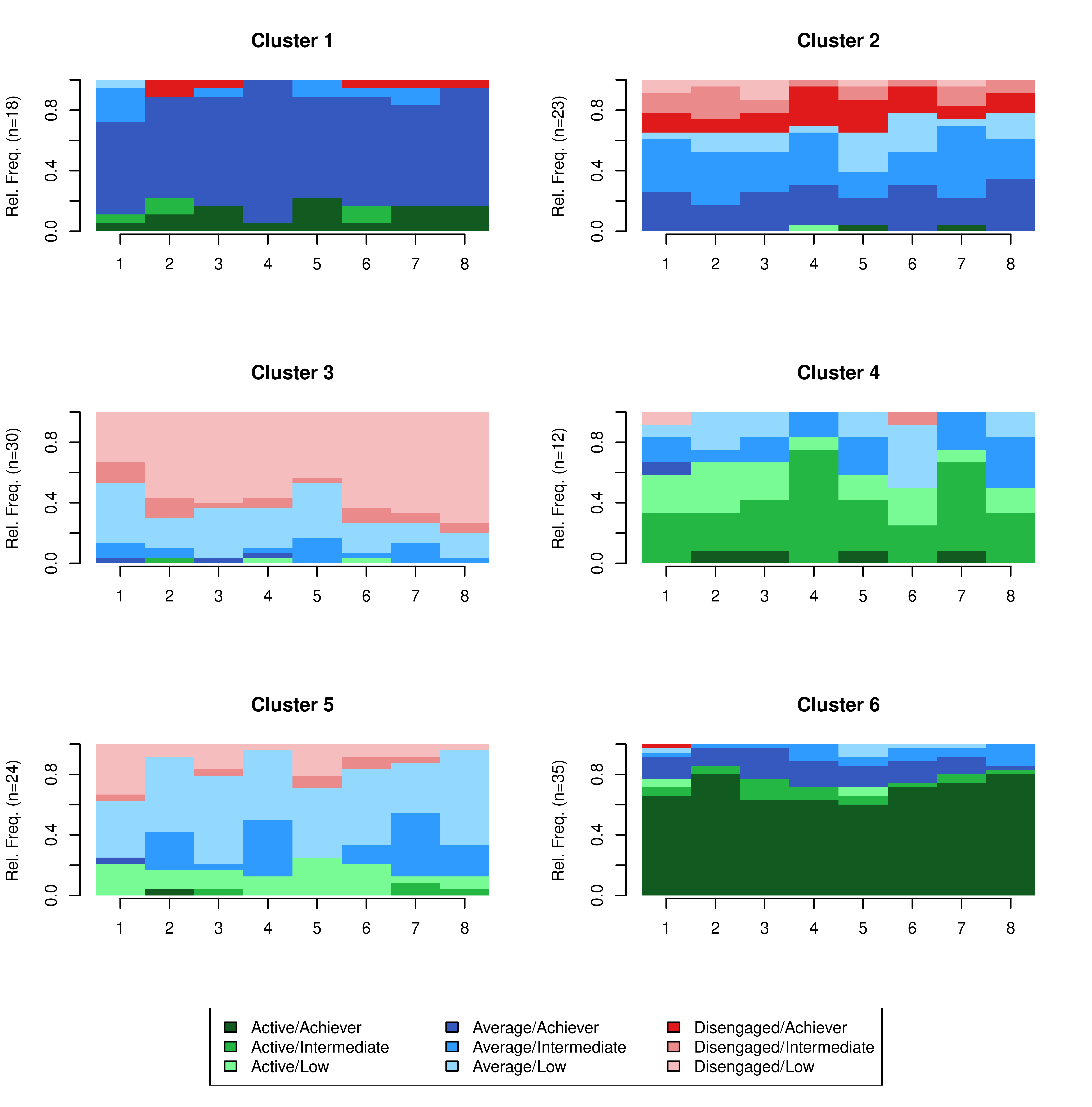
Though there is some evidence of well-defined clusters capturing different engagement and achievement levels over time, a plot such as this can be difficult to interpret, even for a small number of channels and small numbers of per-channel states. A more visually appealing alternative is provided by the stacked state distribution plots below, which shows each individual channel with its own alphabet on the same plot, with one such plot per cluster. This requires supplying a list of the observations ìn each cluster in each channel to the ssp() function to create each plot, with each plot then arranged and displayed appropriately by the function gridplot().
ssp_k <- list()
for(k in 1:6) {
  ssp_k[[k]] <- ssp(list(eng_seq[Cuts == k,],
                         ach_seq[Cuts == k,]),
                    type = "d", border = NA,
                    with.legend = FALSE, title = levels(Groups)[k])
}
gridplot(ssp_k, ncol = 3, byrow = TRUE,
         row.prop = c(0.4, 0.4, 0.2), cex.legend = 0.8)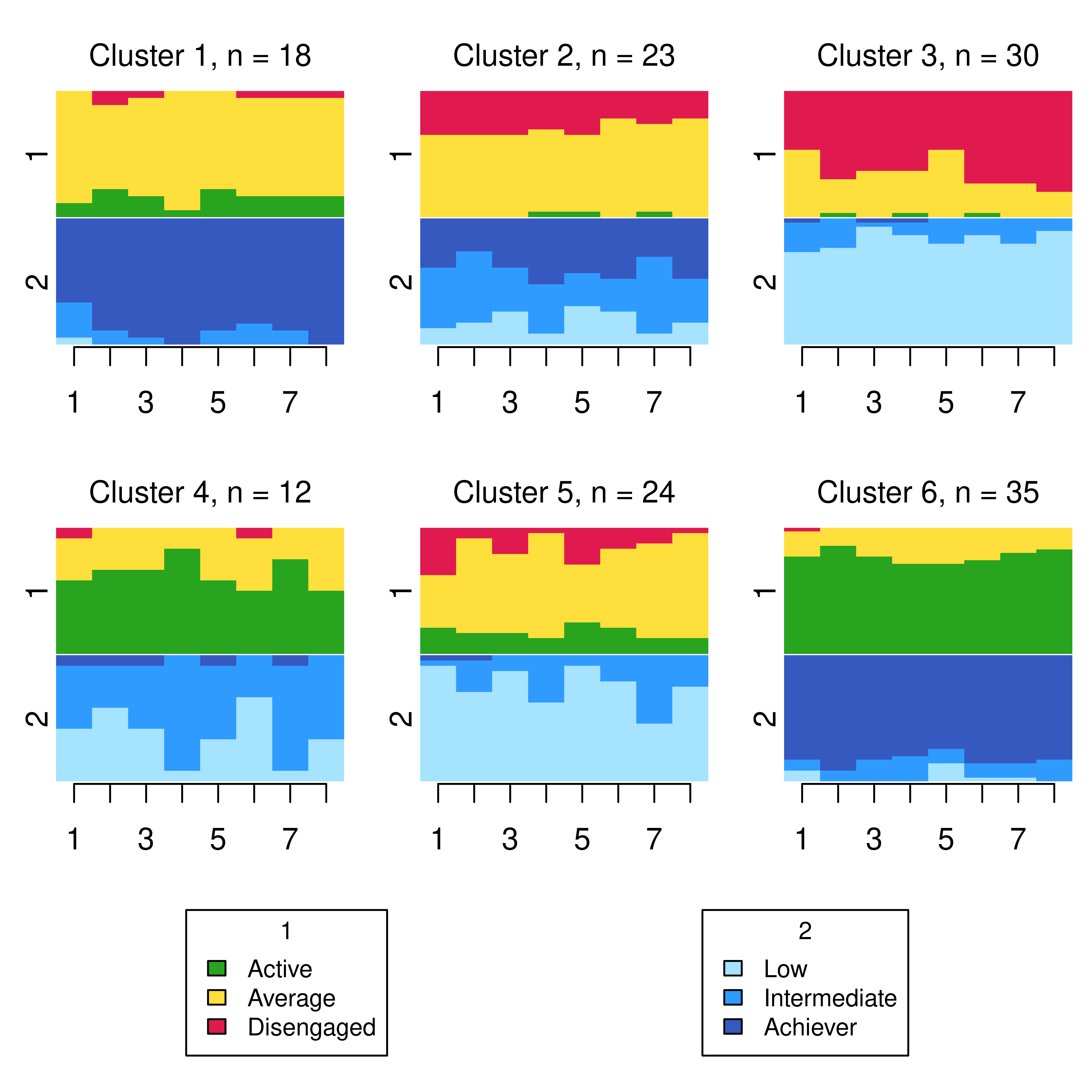
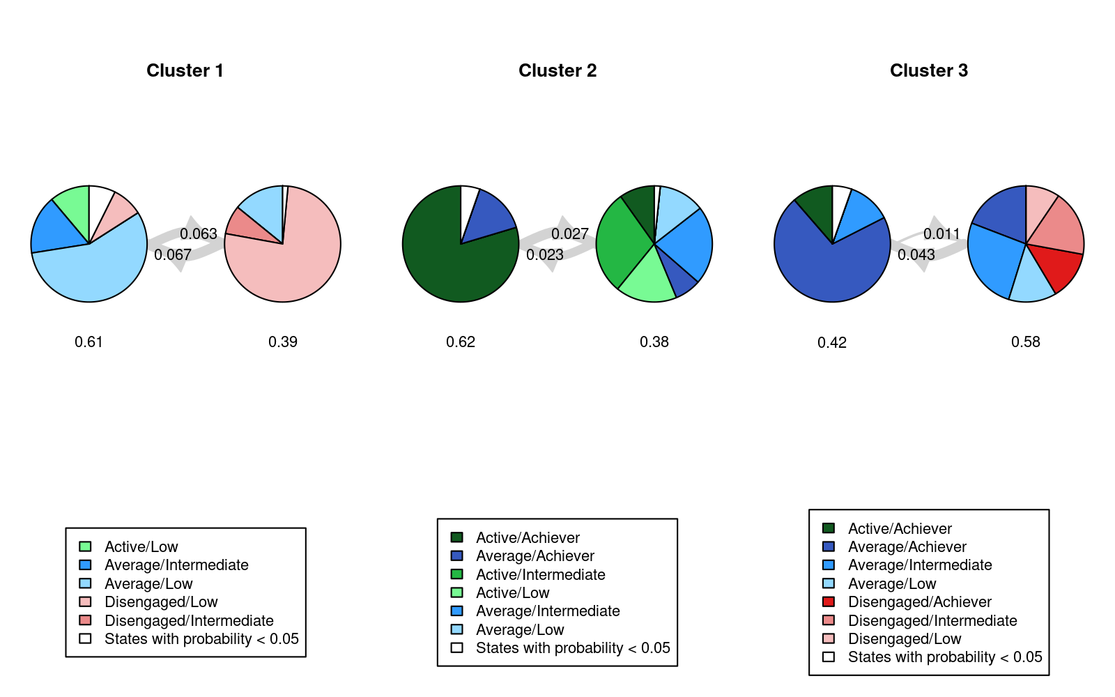
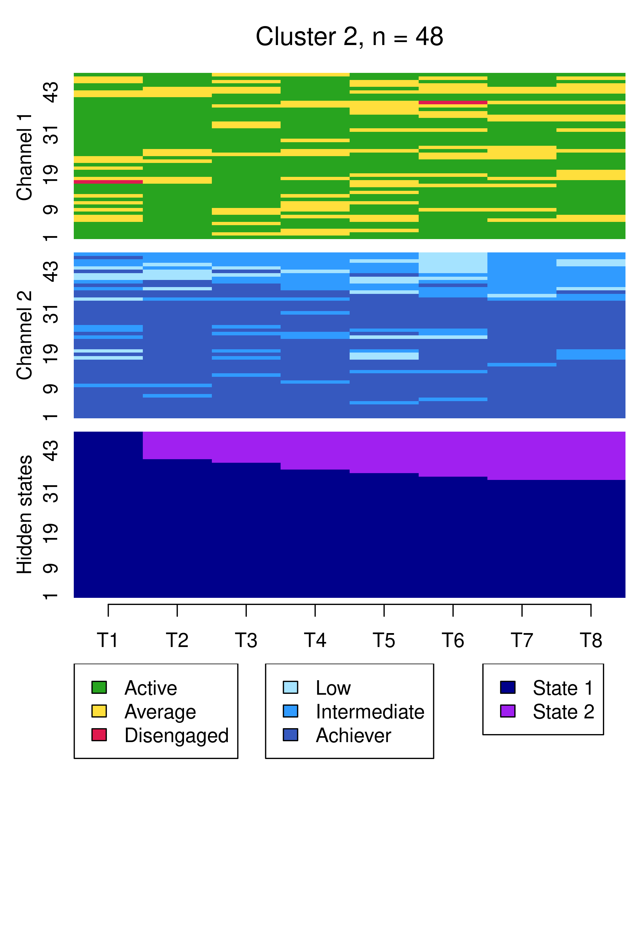
From this plot, we can see six clusters, relating respectively to 1) mostly averagely engaged high achievers, 2) mostly actively engaged intermediate achievers, 3) mostly disengaged intermediate or high achievement, 4) mostly averagely engaged low achievers, 5) mostly disengaged low achievers, and 6) mostly actively engage high achievers. This clustering approach and this set of plots provides quite a granular view of the group structure and interdependencies across channels, which differs somewhat from the clustering solution obtained by the application of MHMMs which now follows.


13.4.6 Incorporating covariates in MHMMs
The BIC can also be used to select the optimal model when different candidate models with different subsets of covariates are fitted. Recall that the clustering and the relation of clusters to covariates is performed simultaneously. Thus, otherwise identical models without dependence on covariates, or using different covariates, may uncover different groupings with different probabilities and hence a different BIC score. Here, we take the optimal model –with three clusters, each with two hidden states, using fixed initial probabilities– and demonstrate how to add and select covariates to make the model more powerful and interpretable. We begin by extracting the covariate information from the original, long format df. For each student, the available time-constant covariates are a numeric variable giving their previous grades from an earlier course, a numeric measure of their attitude towards learning, and their gender (male or female). The order of the rows of cov_df matches the order in the two eng_seq and ach_seq channels.
cov_df <- df |>
  arrange(UserID, Sequence) |>
  filter(!duplicated(UserID)) |>
  select(Prev_grade, Attitude, Gender)
The code below replicates the code used to fit the previously optimal MHMM model, and augments it by providing a data frame (via the data argument, using the cov_df just created) and the corresponding one-sided formula for specifying the covariates to include (via the formula argument). For simplicity, we keep the same number of clusters and hidden states and fit three models (one for each covariate in cov_df). To mitigate against convergence issues, we use the results of the previously optimal MHMM to provide informative starting values.
set.seed(2294)
init_mhmm_1 <- build_mhmm(observations = list(eng_seq, ach_seq),
                          initial_probs = mhmm_fit_i$model$initial_probs,
                          transition_probs = mhmm_fit_i$model$transition_probs,
                          emission_probs = mhmm_fit_i$model$emission_probs,
                          data = cov_df,
                          formula = ~ Prev_grade)
init_mhmm_2 <- build_mhmm(observations = list(eng_seq, ach_seq),
                          initial_probs = mhmm_fit_i$model$initial_probs,
                          transition_probs = mhmm_fit_i$model$transition_probs,
                          emission_probs = mhmm_fit_i$model$emission_probs,
                          data = cov_df,
                          formula = ~ Attitude)
init_mhmm_3 <- build_mhmm(observations = list(eng_seq, ach_seq),
                          initial_probs = mhmm_fit_i$model$initial_probs,
                          transition_probs = mhmm_fit_i$model$transition_probs,
                          emission_probs = mhmm_fit_i$model$emission_probs,
                          data = cov_df,
                          formula = ~ Gender)
We estimate each model 50 + 1 times (first from the starting values we provided and then from 50 randomised values).
mhmm_fit_1 <- fit_model(init_mhmm_1,
                        control_em = list(restart = list(times = 50)))
mhmm_fit_2 <- fit_model(init_mhmm_2,
                        control_em = list(restart = list(times = 50)))
mhmm_fit_3 <- fit_model(init_mhmm_3,
                        control_em = list(restart = list(times = 50)))
Note that in an ideal analysis, however, one would vary the number of clusters and hidden states along with varying sets of covariates and initial probabilities in order to find the model settings which jointly optimise the BIC. Moreover, one is not limited to including only a single covariate; one could specify for example formula = ~ Attitude + Gender, but we omit this consideration here for simplicity. Furthermore, one should check in an ideal analysis that the optimal model was found in a majority of the 51 runs. We did so and can be satisfied that there are no convergence issues. We select among the three models with three different, single covariates using the BIC, and include the previous model with no covariates in the comparison also.
BIC(mhmm_fit_i$model)[1] 3656.949BIC(mhmm_fit_1$model)[1] 3614.673BIC(mhmm_fit_2$model)[1] 3632.004BIC(mhmm_fit_3$model)[1] 3649.353Recalling that lower BIC values are indicative of a better model, we can see that each covariate yields a better-fitting model. Though a better model could be found by adding more covariates or modifying the numbers of clusters and hidden states, we now proceed to interrogate, interpret, and visualise the results of the best model only; namely the MHMM with Prev_grade as a predictor of cluster membership.
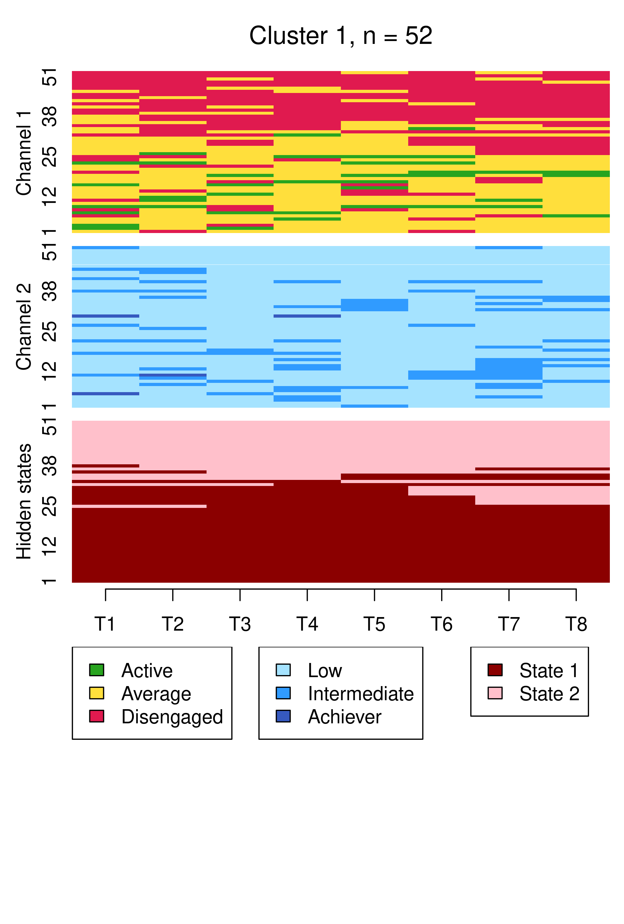
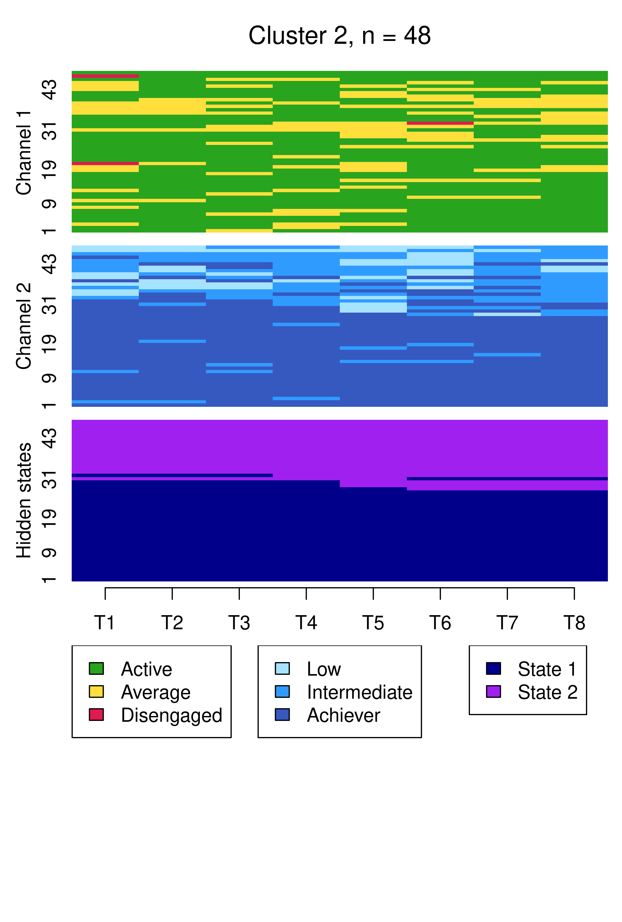
We begin by examining the clusters via sequence index plots using mssplot(), as before, in Figure 13.11.
mssplot(mhmm_fit_1$model,
        plots = "both",
        type = "I",
        sortv = "mds.hidden",
        yaxis = TRUE,
        with.legend = "bottom",
        ncol.legend = 1,
        cex.title = 1.3,
        hidden.states.colors = HIDDEN_STATES)
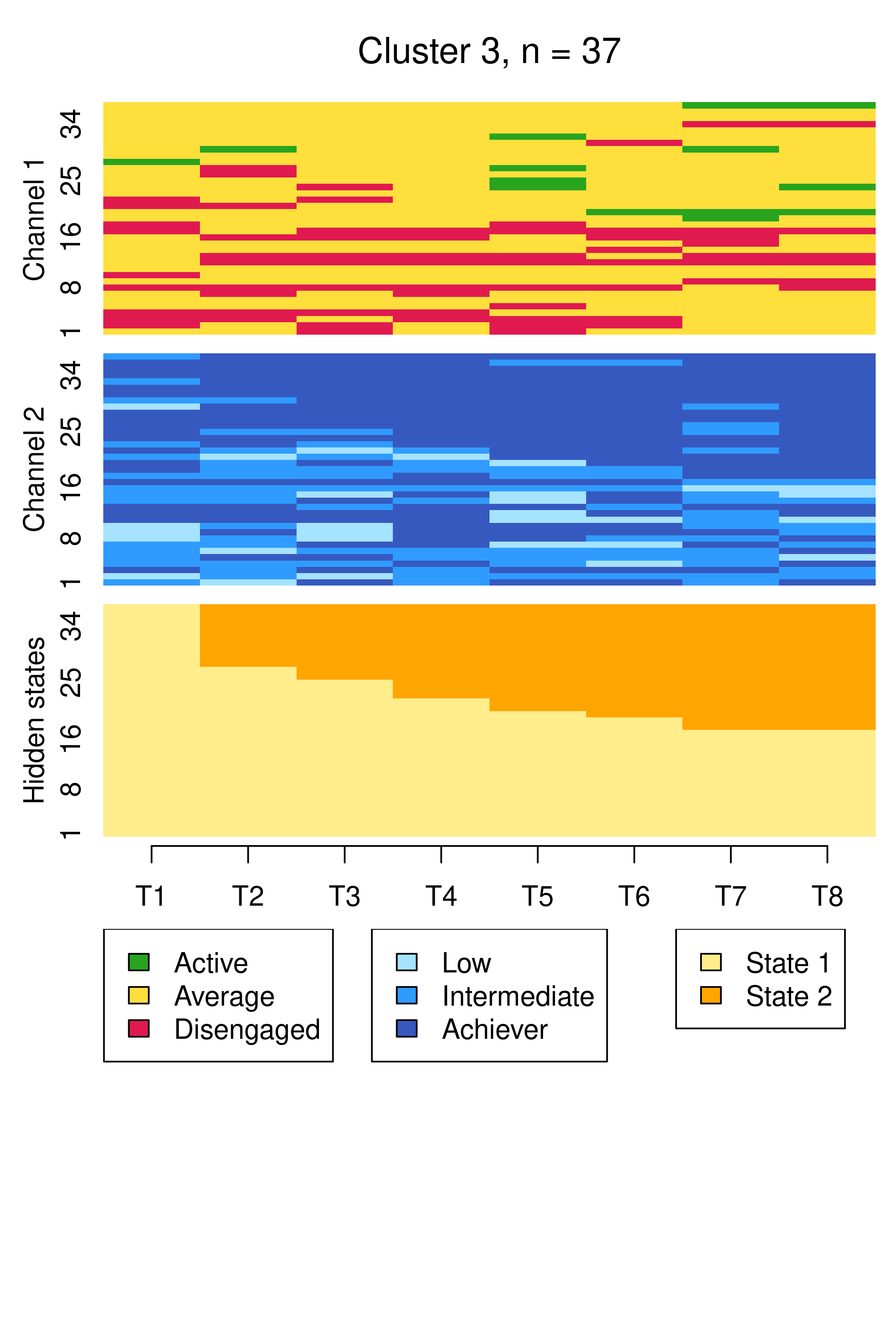
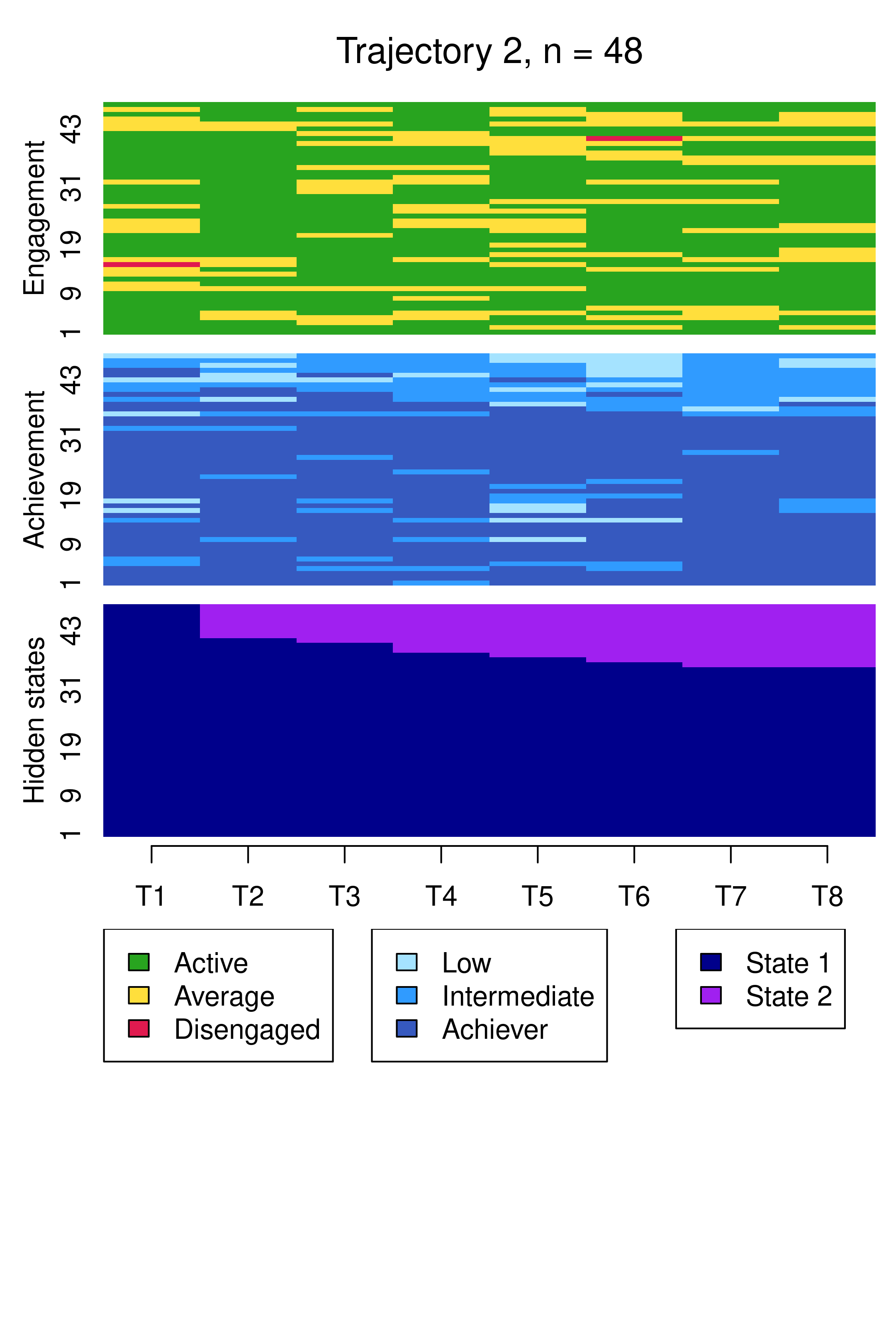
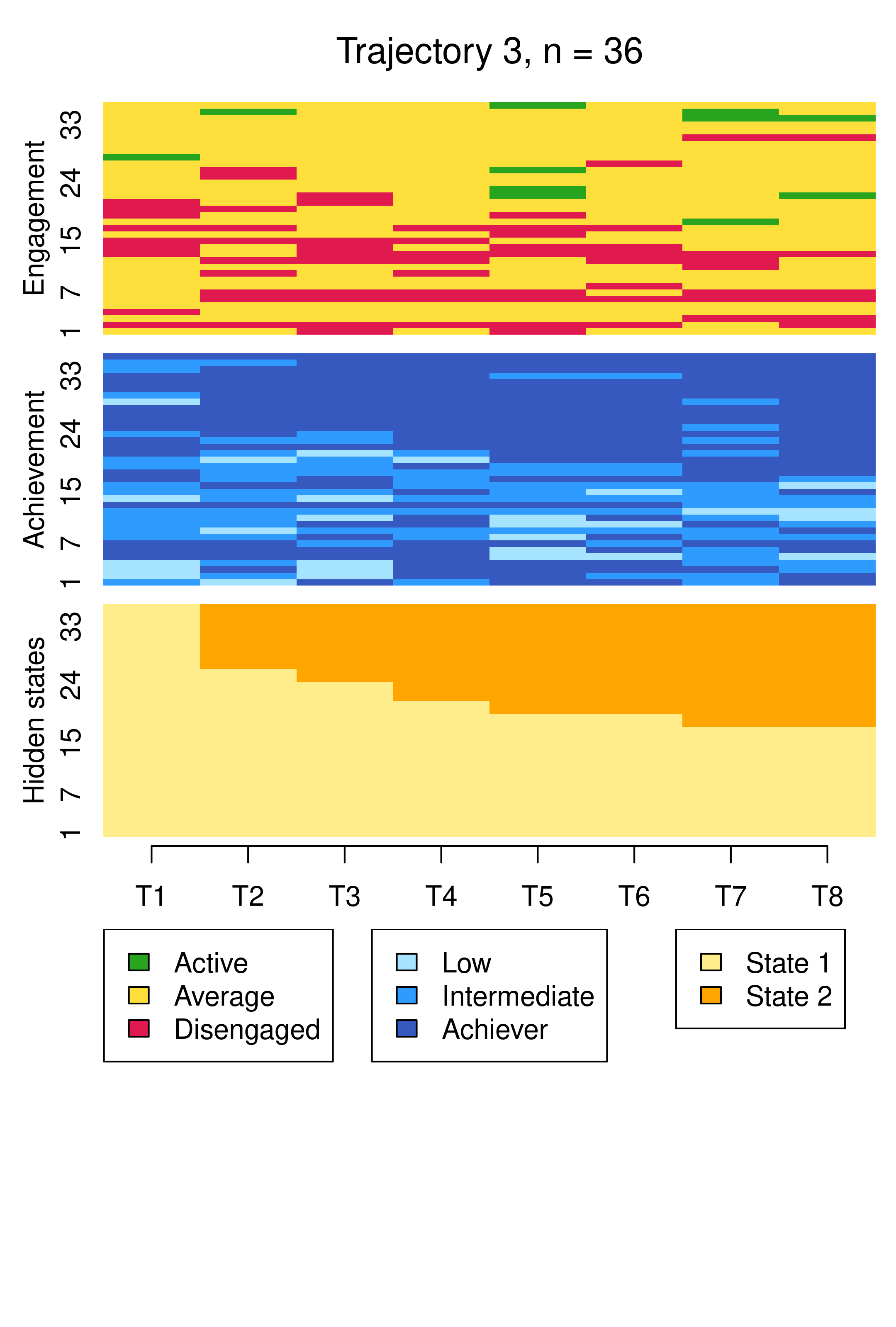
Compared to Figure 13.10, the results are notably similar. One observation previously assigned to the first trajectory is now assigned to the third, but the clusters retain precisely the same interpretations of Cluster 1 being mostly low achievers who move from averagely engaged to disengaged, Cluster 2 being mostly highly engaged high achievers, some of whom transition to being mostly intermediate achievers, and Cluster 3 being most averagely engaged or disengaged high or intermediate achievers, some of whom become more averagely engaged and highly achieving over time. It is worth noting that it is possible for the clusters and the interpretation thereof to change more drastically than this when covariates are added. As the clusters are very similar to what we found before, we give the clusters more informative labels as a reminder:
cluster_names(mhmm_fit_1$model) <- c("LowEngLowAch", "HighEngHighAch", "LowEngHighAch")We now present a summary of the model which shows information about parameter estimates of covariates and prior and posterior cluster membership probabilities, which refer to cluster membership probabilities before or after conditioning on the observed sequences, respectively. In other words, prior cluster membership probabilities are calculated using each individual’s observed covariate values only, while posterior cluster membership probabilities are calculated using individual’s covariate values their observed sequence. In each case, these represent the probabilities of belonging to a particular HMM component in the MHMM mixture.
summary_mhmm_1 <- summary(mhmm_fit_1$model)
summary_mhmm_1
Covariate effects :
LowEngLowAch is the reference.
HighEngHighAch :
Estimate Std. error
(Intercept) -6.253 1.220
Prev_grade 0.817 0.159
LowEngHighAch :
Estimate Std. error
(Intercept) -1.486 0.960
Prev_grade 0.158 0.139
Log-likelihood: -1708.843 BIC: 3614.673
Means of prior cluster probabilities :
LowEngLowAch HighEngHighAch LowEngHighAch
0.40 0.34 0.26
Most probable clusters :
LowEngLowAch HighEngHighAch LowEngHighAch
count 57 48 37
proportion 0.401 0.338 0.261
Classification table :
Mean cluster probabilities (in columns) by the most probable cluster (rows)
LowEngLowAch HighEngHighAch LowEngHighAch
LowEngLowAch 0.98577 0.00702 0.00721
HighEngHighAch 0.00316 0.98499 0.01185
LowEngHighAch 0.01335 0.01552 0.97113We will first interpret the information on prior and posterior cluster membership probabilities and then proceed to interpreting covariate effects. Firstly, the section named Means of prior cluster probabilities gives information on how likely each cluster is in the whole population of students (40% in “LowEngLowAch”, 34% in “HighEngHighAch”, and 26% in “LowEngHighAch”). Secondly, the section Most probable clusters shows group sizes and proportions considering that each student would be classified into the cluster for which they have the highest cluster membership probability. Thirdly, the Classification table shows mean cluster probabilities (in columns) by the most probable cluster (in rows). We can see that the clusters are very crisp (the certainty of cluster memberships are very high) because the membership probabilities are large in the diagonal of the table.
The part titled Covariate effects shows the parameter estimates for the covariates. Interpretation of the values is similar to that of multinomial logistic regression, meaning that we can interpret the direction and uncertainty of the effect –relative to the reference level of “LowEngLowAch” – but we cannot directly interpret the magnitude of the effects. The magnitude of the Prev_grade coefficient is small with respect to its associated standard error, so we can say there is no significant relationship between previous grades and membership of the poorly engaged yet highly achieving “LowEngHighAch”. However, the large positive coefficient in “HighEngHighAch” indicates that students with high previous grades are more likely to belong to the highly engaged high achieving cluster, which makes intuitive sense.
The summary object also calculates prior and posterior cluster memberships for each student. We omit them here, for brevity, but demonstrate that they can be obtained as follows:
prior_prob <- summary_mhmm_1$prior_cluster_probabilities
posterior_prob <- summary_mhmm_1$posterior_cluster_probabilities
Similarly, to obtain the most likely cluster assignment for each student according to the posterior probabilites, we simply need to access the most_probable_cluster element from the summary object (summary_mhmm_1). As per the Groups vector defined in the earlier distance-based clustering analysis, we show the assignments for the first 5 students only below, for brevity.
cluster_assignments <- summary_mhmm_1$most_probable_cluster
head(cluster_assignments, 5)
[1] LowEngHighAch LowEngLowAch LowEngLowAch HighEngHighAch LowEngLowAch
Levels: LowEngLowAch HighEngHighAch LowEngHighAchIf we are interested in getting the most probable path of hidden states for each student, we may use the hidden_paths() function from seqHMM and pass the MHMM model as an argument (mhmm_fit_1$model). We then need to convert it to the long format to get a row per student and timepoint and then we extract only the value column to get only the hidden state. We can then assign the resulting vector to a column (e.g., HiddenState) in the original dataframe which follows the same data order.
df$HiddenState <- hidden_paths(mhmm_fit_1$model) |>
  pivot_longer(everything()) |> pull(value)
head(df$HiddenState)
[1] LowEngHighAch:State 1 LowEngHighAch:State 1 LowEngHighAch:State 2
[4] LowEngHighAch:State 2 LowEngHighAch:State 2 LowEngHighAch:State 2
8 Levels: LowEngLowAch:State 1 LowEngLowAch:State 2 ... %It is good to be aware that the most probable cluster according to posterior cluster probabilities may not always match with the cluster producing the single most probable path of hidden states. This is because the posterior cluster probabilities are calculated based on all of the possible hidden state paths generated from that cluster, while the single most probable path of hidden states may sometimes come from a different cluster.
Lastly, we advise readers to consult Chapter 12 for more examples of interpreting covariate effects in the context of MHMM models.
13.5 Discussion
This chapter has provided an introduction to multi-channel sequence analysis, a method that deals with the analysis of two or more synchronised sequences. Throughout this chapter, we have highlighted the growing significance of multi-channel sequence analysis in educational research. While earlier chapters in this book focused on sequence analysis of learner-related data, this method presents a suitable approach to leverage the increasing availability of student multimodal temporal data. Our review of the existing literature that has utilised multi-channel sequence analysis concluded that the applications of this method within educational research are still relatively scarce. However, the potential of this framework is immense, as it opens up new possibilities to address the challenges posed by the complex and dynamic nature of educational data.
In the tutorial part of the chapter, we examined a case study on students’ online engagement and academic achievement to demonstrate how multi-channel sequence analysis can reveal valuable insights into the longitudinal associations between these constructs. The identification of distinct trajectories through mixture hidden Markov models allows for a deep understanding of how both constructs evolve together over time and the distance-based clustering approach offers an alternative perspective on the group structure within these data. The step-by-step tutorial on implementing multi-channel sequence analysis with R according to both clustering frameworks provides readers with practical guidance to explore and apply these methods in their own research. Armed with this knowledge, researchers and educators can unlock valuable insights from their data and make informed decisions to support student learning and success.
Markovian models are relatively scalable and can be used to cluster large sequence data. See, e.g., [36] for scalability in terms of hidden states and time points in hidden Markov models. In terms of the number of sequences, computations can be easily parallelised; see, e.g., [19]. Then again, unlike data-mining type sequence analysis, probabilistic models require making assumptions about the data-generating mechanisms which may not always be realistic (such as time-homogeneity or the Markov property itself [19]. Furthermore, analysis of complex multi-channel sequence data can be very time consuming [6, 37]. Although we have highlighted the advantages of the model-based Markovian approach, particularly with regard to the ability to incorporate covariates as predictors of cluster membership, it is difficult to say if one approach is definitively better than the other for all potential use-cases. Although information criteria such as the BIC or cross-validation can be used to guide the choice of MHMM, particularly regarding the choice of the number of clusters (and numbers of hidden states within each cluster, and/or initial/transition/emission probabilities), we did not comprehensively do so here. Rather, we opted for three clusters, each with two hidden states, in both applications of MHMM herein, and only considered different initial probability settings and different covariates to arrive at the best model in terms of BIC. In an ideal analysis, one would compare different MHMM fits with different numbers of clusters and hidden states, different restrictions on the probabilities, and different covariates to arrive at an optimal model in terms of BIC or other model selection criteria.
Conversely, the choice of six clusters for the hierarchical clustering solution was arrived at in a different fashion, driven by the average silhouette width cluster quality measure. Indeed, the BIC cannot be used to choose the number of clusters with hierarchical clustering, nor can it be used to compare a hierarchical clustering solution with MHMM. However, it is interesting to note that the six clusters obtained by hierarchical clustering map reasonably well to the six hidden states of the MHMM solutions. As examples, considering the MHMM with fixed initial probabilities, one could say that clusters 4 and 5 of the hierarchical clustering solution, capturing averagely engaged and disengaged low achievers respectively, matches the two hidden states of the first MHMM cluster, while clusters 2 and 6, capturing actively engaged intermediate and high achievers respectively, matches the two hidden states of the second MHMM cluster.
Overall, we encourage readers to further explore the potential of multi-channel sequence analysis, the merits of both clustering approaches, and broader implications in the field of education by diving into the recommended readings. The next section provides a list of valuable resources for readers to expand their knowledge on the topic.
13.6 Further readings
For more thorough presentations and comparisons of different options for the distance-based analysis of multi-channel sequences, we recommend the text book by Struffolino and Raab [38] and articles by Emery and Berchtold [8] and Ritschard et al. [13]. For assessing whether sequences in different channels are associated to the extent of needing joint analysis, Piccarreta and Elzinga [39, 40] have proposed solutions for quantifying the extent of association between two or more channels using Cronbach’s \(\alpha\) and principal component analysis.
For general presentations of the MHMM for multi-channel sequences, see the chapter by Vermunt et al. [41] and the article by Helske and Helske [19]. For further examples and tips for visualization of multi-channel sequence data and estimation of Markovian models with the seqHMM package, see the seqHMM vignettes [42, 43].
To learn how to combine distance-based sequence analysis and hidden Markov models for the analysis of complex multi-channel sequence data with partially missing observations, see the chapter by Helske et al. [6].
14 Acknowledgements
SH was supported by the Academy of Finland (decision number 331816), the Academy of Finland Flagship Programme (decision number 320162), and the Strategic Research Council (SRC), FLUX consortium (decision numbers: 345130 and 345130). MS was supported by the Academy of Finland (TOPEILA: Towards precision education: Idiographic learning analytics, grant 350560).
References
1.
Saqr M, Nouri J, Fors U (2019) Time to focus on the temporal dimension of learning: A learning analytics study of the temporal patterns of students’ interactions and self-regulation. International Journal of Technology Enhanced Learning 11:398. https://doi.org/10.1504/ijtel.2019.102549
2.
Saqr M, López-Pernas S (2023) The temporal dynamics of online problem-based learning: Why and when sequence matters. International Journal of Computer-Supported Collaborative Learning 18:11–37. https://doi.org/10.1007/s11412-023-09385-1
3.
Saqr M, López-Pernas S, Helske S, Durand M, Murphy K, Studer M, Ritschard G (2024) Sequence analysis in education: Principles, technique, and tutorial with r. In: Saqr M, López-Pernas S (eds) Learning analytics methods and tutorials: A practical guide using R. Springer
4.
López-Pernas S, Saqr M (2024) Modeling the dynamics of longitudinal processes in education. A tutorial with r for the VaSSTra method. In: Saqr M, López-Pernas S (eds) Learning analytics methods and tutorials: A practical guide using R. Springer, pp in–press
5.
Helske J, Helske S, Saqr M, López-Pernas S, Murphy K (2024) A modern approach to transition analysis and process mining with markov models: A tutorial with R. In: Saqr M, López-Pernas S (eds) Learning analytics methods and tutorials: A practical guide using R. Springer, pp in–press
6.
Helske S, Helske J, Eerola M (2018) Combining sequence analysis and hidden Markov models in the analysis of complex life sequence data. In: Life course research and social policies. Springer International Publishing, pp 185–200
7.
Eisenberg-Guyot J, Peckham T, Andrea SB, Oddo V, Seixas N, Hajat A (2020) Life-course trajectories of employment quality and health in the U.S.: A multichannel sequence analysis. Social Science & Medicine 264:113327. https://doi.org/10.1016/j.socscimed.2020.113327
8.
Emery K, Berchtold A (2022) Comparison of two approaches in multichannel sequence analysis using the Swiss Household Panel. Longitudinal and Life Course Studies 1–32. https://doi.org/10.1332/175795921x16698302233894
9.
Gauthier J-A, Widmer ED, Bucher P, Notredame C (2010) Multichannel sequence analysis applied to social science data. Sociological Methodology 40:1–38. https://doi.org/10.1111/j.1467-9531.2010.01227.x
10.
Saqr M, López-Pernas S, Helske S, Hrastinski S (2023) The longitudinal association between engagement and achievement varies by time, students’ profiles, and achievement state: A full program study. Computers & Education 199:104787. https://doi.org/10.1016/j.compedu.2023.104787
11.
Winne PH (2020) Construct and consequential validity for learning analytics based on trace data. Computers in Human Behavior 112:106457. https://doi.org/10.1016/j.chb.2020.106457
12.
Murphy K, López-Pernas S, Saqr M (2024) Dissimilarity-based cluster analysis of educational data: A comparative tutorial using R. In: Saqr M, López-Pernas S (eds) Learning analytics methods and tutorials: A practical guide using R. Springer, pp in–press
13.
Ritschard G, Liao TF, Struffolino E (2023) Strategies for multidomain sequence analyis in social research. Sociological Methodology 53:288–322. https://doi.org/10.1177/0081175023116383
14.
Pollock G (2007) Holistic trajectories: A study of combined employment, housing and family careers by using multiple-sequence analysis. Journal of the Royal Statistical Society: Series A (Statistics in Society) 170:167–183
15.
Saqr M, López-Pernas S, Jovanović J, Gašević D (2023) Intense, turbulent, or wallowing in the mire: A longitudinal study of cross-course online tactics, strategies, and trajectories. The Internet and Higher Education 57:100902
16.
Bouguettaya A, Yu Q, Liu X, Zhou X, Song A (2015) Efficient agglomerative hierarchical clustering. Expert Systems with Applications 42:2785–2797. https://doi.org/https://doi.org/10.1016/j.eswa.2014.09.054
17.
Gilpin S, Qian B, Davidson I (2013) Efficient hierarchical clustering of large high dimensional datasets. In: Proceedings of the 22nd ACM international conference on information & knowledge management. Association for Computing Machinery, New York, NY, USA, pp 1371–1380
18.
Studer M (2013) WeightedCluster library manual: A practical guide to creating typologies of trajectories in the social sciences with R. LIVES. https://doi.org/10.12682/LIVES.2296-1658.2013.24
19.
Helske S, Helske J (2019) Mixture hidden Markov models for sequence data: The seqHMM package in R. Journal of Statistical Software 88: https://doi.org/10.18637/jss.v088.i03
20.
Schwarz GE (1978) Estimating the dimension of a model. The Annals of Statistics 6:461–464. https://doi.org/10.1214/aos/1176344136
21.
22.
Murphy K, Murphy TB, Piccarreta R, C. GI (2021) Clustering longitudinal life-course sequences using mixtures of exponential-distance models. Journal of the Royal Statistical Society: Seria A (Statistics in Society) 184:1414–1451
23.
Studer M (2018) Divisive Property-Based and fuzzy clustering for sequence analysis. In: Ritschard G, Studer M (eds) Sequence analysis and related approaches: Innovative methods and applications. Springer International Publishing, Cham, pp 223–239
24.
Helske S, Helske J, Chihaya GK (2023) From sequences to variables: Rethinking the relationship between sequences and outcomes. Sociol Methodol 00811750231177026. https://doi.org/10.1177/00811750231177026
25.
Dayton CM, Macready GB (1988) Concomitant-variable latent-class models. Journal of the American Statistical Association 83:173–178
26.
Murphy K, Murphy TB (2020) Gaussian parsimonious clustering models with covariates and a noise component. Advances in Data Analysis and Classification 14:293–325
27.
Törmänen T, Järvenoja H, Saqr M, Malmberg J, Järvelä S (2022) A person-centered approach to study students’ socio-emotional interaction profiles and regulation of collaborative learning. Frontiers in Education 7: https://doi.org/10.3389/feduc.2022.866612
28.
Törmänen T, Järvenoja H, Saqr M, Malmberg J, Järvelä S (2022) Affective states and regulation of learning during socio-emotional interactions in secondary school collaborative groups. British Journal of Educational Psychology 93:48–70. https://doi.org/10.1111/bjep.12525
29.
Ouyang F, Xu W, Cukurova M (2023) An artificial intelligence-driven learning analytics method to examine the collaborative problem-solving process from the complex adaptive systems perspective. International Journal of Computer-Supported Collaborative Learning 18:39–66. https://doi.org/10.1007/s11412-023-09387-z
30.
Lopez-Pernas S, Saqr M (2021) Bringing synchrony and clarity to complex multi-channel data: A learning analytics study in programming education. IEEE Access 9:166531–166541. https://doi.org/10.1109/access.2021.3134844
31.
Bacci S, Bertaccini B (2022) A mixture hidden Markov model to mine students’ university curricula. Data 7:25. https://doi.org/10.3390/data7020025
32.
Liu B, Widener MJ, Smith LG, Farber S, Minaker LM, Patterson Z, Larsen K, Gilliland J (2021) Disentangling time use, food environment, and food behaviors using multi-channel sequence analysis. Geographical Analysis 54:881–917. https://doi.org/10.1111/gean.12305
33.
Chan C, Chan GC, Leeper TJ, Becker J (2021) Rio: A Swiss-army knife for data file I/O
34.
Wickham H, Averick M, Bryan J, Chang W, McGowan LD, François R, Grolemund G, Hayes A, Henry L, Hester J, Kuhn M, Pedersen TL, Miller E, Bache SM, Müller K, Ooms J, Robinson D, Seidel DP, Spinu V, Takahashi K, Vaughan D, Wilke C, Woo K, Yutani H (2019) Welcome to the tidyverse. Journal of Open Source Software 4:1686. https://doi.org/10.21105/joss.01686
35.
Gabadinho A, Ritschard G, Müller NS, Studer M (2011) Analyzing and visualizing state sequences in R with TraMineR. Journal of Statistical Software 40: https://doi.org/10.18637/jss.v040.i04
36.
Rabiner LR (1989) A tutorial on hidden Markov models and selected applications in speech recognition. Proceedings of the IEEE 77:257–286. https://doi.org/10.1109/5.18626
37.
Berchtold A (2004) Optimization of mixture models: Comparison of different strategies. Computational Statistics 19:385–406. https://doi.org/10.1007/bf03372103
38.
Raab M, Struffolino E (2022) Sequence analysis. SAGE Publications
39.
Piccarreta R, Elzinga CH (2013) Mining for association between life course domains. In: Contemporary issues in exploratory data mining in the behavioral sciences. Routledge, pp 212–242
40.
Piccarreta R (2017) Joint sequence analysis: Association and clustering. Sociological Methods & Research 46:252–287
41.
Vermunt JK, Tran B, Magidson J (2008) Latent class models in longitudinal research. Handbook of longitudinal research: Design, measurement, and analysis 373–385
42.
Helske S (2017) Visualization tools in the seqHMM package
43.
Helske S (2017) Examples and tips for estimating markovian models with seqHMM