print("Hello, world!")[1] "Hello, world!"R is a free, versatile, and open source programming language and software environment specifically designed for statistical computing and data analysis. R has a vast library of packages that enable data manipulation, visualization, modeling and machine learning [1]. Such a wealth of packages enable a wide range of functionalities that saves the users time, effort or the need to write complex code. The fact that R is freely available makes all these functionalities accessible to all. R has a large community of developers, users and researchers who support the development of the platforms as well as provide support and shared knowledge on popular sites such as StackExchange. Thereupon, R is becoming an increasingly popular choice for students, researchers and data scientists [2].
Being open source and accessible to researchers, several packages are added continuously to expand the possibilities and functions that R offers. Some of the R packages included in this book have been added by researchers during the last few years to address contemporary scientific problems and state-of-the-art innovations [3]. For example, R software packages for the analysis of psychological networks were developed in the past five years and ever since have grown tremendously due to contributions from a large base of researchers [4].
Although many of the methods described in this book can be implemented with other software tools, it is hard to find a comprehensive platform that can be used to perform practically all the existing learning analytics methods with such maturity, performance and range of possibilities. For instance, Social Network Analysis (SNA) can be performed with several programming languages (e.g., Python) and desktop software applications (e.g., Gephi) [5]. However, both options provide limited capabilities compared to what R provides for the analysis of SNA. This includes a wider range of SNA centrality measures, mathematical models, community finding algorithms and generative models. Sequence analysis is another example in which the possibilities offered by R are hard to match with other software solutions.
This book does not make any assumptions about the superiority of R over any other platform. Other languages and software platforms are indeed very helpful and have vast capabilities for researchers. For instance, Python has remarkable tools for machine learning and Gephi offers beautiful graphics for the visualization of networks. Oftentimes, readers may need to learn or use other tools to do specific tasks. Put another way, where R offers a rich toolset for researchers, there is a space for other tools that researchers can use to accomplish certain tasks. In summary, investing time in learning R is a worthwhile endeavor that helps interested researchers to perform and expand their research skills and toolset. Since R is a large platform, it represents a doorway to the vast capabilities of its ever expanding repertoire of functions and packages.
The goal of programming is to write, i.e. code, a program that performs a desired task. A program consists of several commands, each of which does something very simple. In the statistics and data analysis context, R is typically used to write short programs called scripts. R is therefore not intended for developing games or other complicated programs. R is also not a language originally intended for web programming, although with the right packages you can also make web applications with R.
R is a high-level programming language. This means that there are many ready-made commands in R, which have much more code “underneath” that the R programmer does not have to touch. For example, a statistical t-test requires several mathematical intermediate steps, but an R programmer can perform the test with a single command (t.test) that provides all the necessary computations and information about the test.
The best way to learn how to use and program R code is by doing. This text has R code embedded between the text in gray boxes, as in the example below. Lines starting with two hashes, i.e. ##, are not code, but output generated by running the code. Let’s first take the classic “Hello, world!” command as an example:
print("Hello, world!")[1] "Hello, world!"The print function prints the given text to the console. It is convenient, for example, for testing the operation of a program and monitoring the progress of a longer program. R can also be used as a calculator. In the example below, we calculate the price of a product after a 35% discount that was originally priced at 80 euros.
80 * (1 - 0.35)[1] 52However, running individual commands is usually not useful unless the results can be saved somewhere. In programming languages, data is stored in variables, which you will become familiar with later.
R has a large array of tools and integrated development environments (IDEs) that make writing and managing code easier and more accessible. The most widely used R IDE is RStudio, which is a free open source software that — similarly to R — runs on all major operating systems [6]. RStudio provides a comprehensive and user-friendly interface for writing, running, and debugging R code, which makes it easier for users to get started and become more productive. Together, R and RStudio allow for the creation of reproducible research. The code and results can be easily shared and replicated, making R and RStudio great tools for collaboration and transparency.
R and RStudio can be very useful in analyzing and visualizing different types of data. This can help researchers, educators and administrators make data-driven decisions and improve the learning experience for students. Whether you are analyzing student performance, demographic data, or tracking the effectiveness of instructional interventions, R and RStudio provide a flexible and efficient platform for achieving your goal.
First install R (step 1) and then RStudio Desktop for your operating system. R and RStudio are available for many operating systems. The interface of RStudio shown in Figure 3.1 has the following default components:
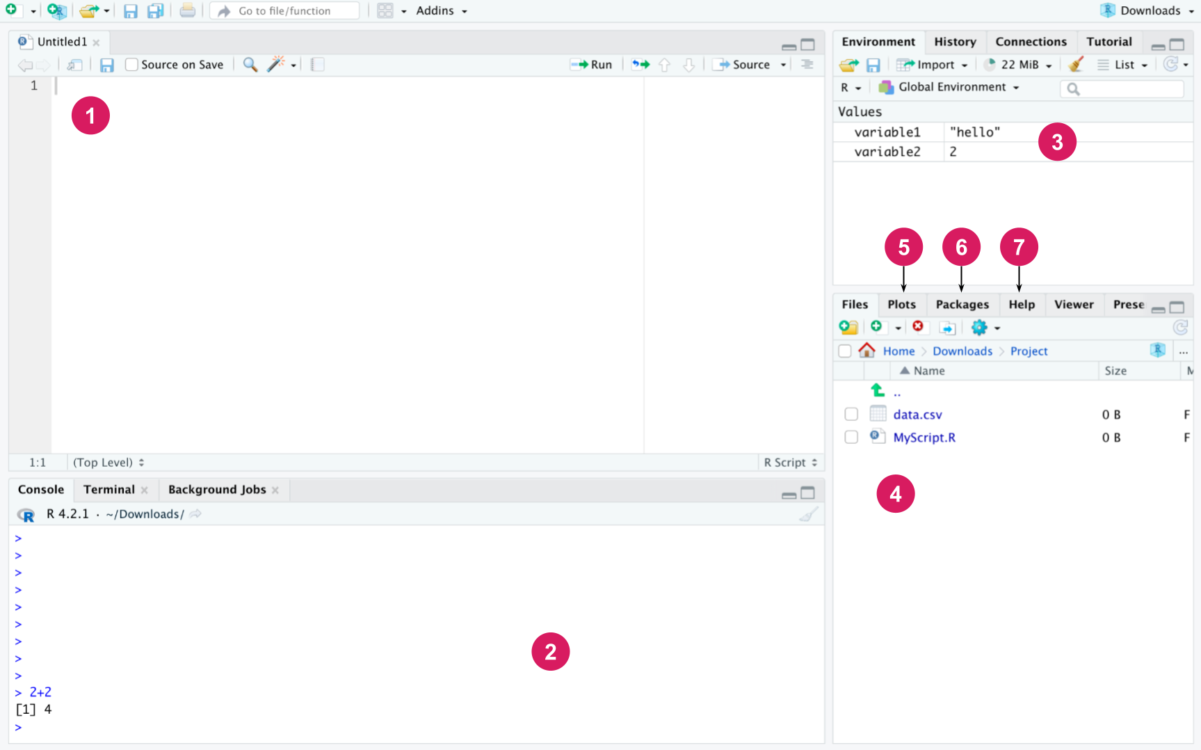
Editor: The editor is used to write files containing R code, i.e., R scripts. Scripts will be introduced later, but they are simply a collection of R commands that carry out a specific task when placed together, for example analyze the data of a research project or draw figures of the finished results. A new script can be opened from the “File” menu by selecting “New File” and then “R script”. The same can be accomplished via a keyboard shortcut by pressing Ctrl + Shift + N on Windows and Linux. On macOS, users can use Cmd + Shift + N. Also, see the “Keyboard Shortcuts Help” under the “Tools” menu for all the shortcuts available. The code written in the editor can be run line by line by pressing Ctrl + Enter at the line. Several lines can also be selected and run at once. The Source button at the top runs all the code in the current file. R scripts can be saved just like other files and their file extension is .R. All the code you use to analyze your data should be written in scripts. When you save your code in this way, the next time you can simply run the script to perform the desired task instead of rewriting the code from scratch.
Console: R commands are executed in the console. If the code written in the editor is run, RStudio automatically executes the commands in the console. In the console, just pressing Enter is enough to execute a line of code. You can try to write a calculation in the console, such as 2 * 3 and press Enter, and the result will be printed in the console. You can also write code in the editor and press Ctrl + Enter to accomplish the same result. Possible messages, warnings and errors are also printed into the console. The main difference between the console and the editor is that the commands written in the console are not saved in any file. So if you want to keep your code, it should be written in the editor and saved in a script file. Commands made during the same session can be scrolled in the console with the up and down arrows. In addition, the command history can be viewed in the History tab in RStudio.
Workspace: Displays the variables in the current working environment of the R session.
Files: Shows the directory structure of the operating system, by default the working directory.
Plots: Graphics drawn with R appear here.
Packages: Here you can manage the installed packages (instructions for installing the packages are below).
Help: Here you can browse the R manual with instructions for every R command. You can try running the ?print command in the editor or console, which opens the help page for the print function.
As the word “script” already suggests, data analysis often requires a “script” of various steps, such as reading measurements from a file, organizing a table, or describing the results of an analysis, for example by calculating the averages of different sample groups and drawing figures. Writing the R commands that perform these steps in a script provides a documentation of how the analysis was done, and it’s also easy to come back to and possibly add a few additional steps, such as performing a t-test. The script file is also easy to share with others who work with similar data analysis tasks, because with small modifications (file names, table structure) the same code also works for different datasets and workflows. Comments are often used inside the code. Comments are text written along the R commands, which are not written in a programming language, and which are ignored when running the code. The purpose of comments is to describe the behavior and purpose of the code. It is good to practice to comment your own code from the beginning, even if the code for the first tasks is very simple. In R, comments are marked with the ## symbol.
## Assign arbitrary numbers to two variables
x <- 3
y <- 5
## Sum of two variables
z <- x + y
## Print the results
z
[1] 8While scripts can only store code and comments, a more comprehensive format called R Markdown is also available in RStudio. R Markdown is an extension of the Markdown markup language that allows users to create dynamic reports and interactive notebooks that can integrate text, code, and visualizations. R Markdown documents are created in a plain text format and can be rendered into various output formats, such as HTML, PDF, Word, or even presentations. To create a new R Markdown document in RStudio, go to the “File” menu, select “New File” and finally “R Markdown”. In the dialog that opens, choose the output format you want to use, and give your document a title. Figure 3.2 shows the RStudio editor panel for a default R Markdown document of R Studio.
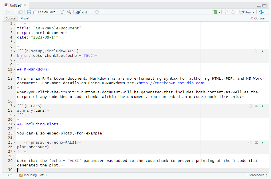
The YAML metadata wrapped between the --- delimiters at the top of the document can be used to customize the output and contents in various ways. For example, you can change the title, author, or add a table of contents. In this example we have defined the title, the output format (HTML) and the date, but many more options are available besides these. Use Markdown syntax to format your text, and enclose your R code in code chunks with the ```{r} and ``` tags which can also be provided other options. For example, our first code chunk has been given the label setup and the following option include = FALSE means that this chunk will be executed but its output will not be printed into the final document. Within the chunk, a global knitr option is set so that all code chunks will print (echo) their output by default. You can also use inline chunks to quickly reference the results of computations or other R objects. Some examples of standard markdown syntax in the document are second level headers marked with ## (note that # is not used for comments in an R Markdown document) and bold text denoted by wrapping the text with **. Once you are satisfied with your document, you can render it into the chosen output format by clicking the “Knit” button in RStudio, or use the keyboard shortcut “Ctrl + Shift + K”. Figure 3.3 shows the corresponding rendered HTML document.
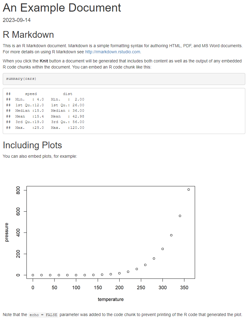
This simple example shows only a fraction of the full features of R Markdown documents and the Markdown syntax. R Markdown is a powerful tool for creating reproducible research reports, teaching materials, or even websites. It allows users to integrate code and output seamlessly into their written work, making it easier to share and reproduce analyses. As an alternative to R Markdown documents, R Studio also supports the creation of R Notebooks, which are in essence interactive R Markdown documents. R Notebooks can be useful for example when the goal is not to produce one comprehensive analysis report but instead to keep track of the code and try out various approaches to a problem interactively. For an in-depth guide to R Markdown, see [7] which is also freely available online at https://bookdown.org/yihui/rmarkdown/.
Code development typically follows similar steps:
Along with this material, many packages include a “Cheat Sheet” as a summary of basic tasks and functions related to the package. Cheat sheets provide a quick and easy reference for checking how something is done in R if you don’t remember it by heart. There are cheat sheets for various R packages and other entities on the Internet e.g., the base R cheat sheet, or the tidyr [8] cheat sheet.
In addition to the basic commands presented in this chapter of the book, practical R programming relies to a great extent on the use of various packages developed by the scientific community. Packages are collections of code that contain new functions, classes and data, i.e., they extend R. Most R packages are available from the Comprehensive R Archive Network (CRAN). They can be installed with the install.packages() function, or via RStudio’s installation window which in practice calls the install.packages() function. You can also install several packages at once. The command below installs the dplyr [9] and tidyr packages:
install.packages(c("dplyr", "tidyr"))In order to use the commands contained in an R package, the package must be installed and attached to the R workspace. This is done with the library() command:
library("tidyr")Now that the tidyr package is loaded, we can use the commands it provides, for example to manage the learning analytics data in data frame format that we will address later. If you don’t want to attach the entire package, you can use individual commands from packages with the format name_of_the_package::name_of_the_command().
Basic operations in R consist of arithmetic operations, logical operations, and assignment. In addition, there are several commands that are often helpful when starting a new project or managing the working directory. For example, the current working directory can be obtained with the following command:
getwd()[1] "/home/sonsoles/labook/chapters/ch03-intro-r"R can be used to compute basic arithmetic operations such as addition (+), subtraction (-), multiplication (*), division (/), and exponentiation (^). These operations follow standard precedence rules, and additional brackets can be added to control the evaluation order if needed.
1 + 1 ## Addition[1] 22 - 1 ## Subtraction[1] 12 * 4 ## Multiplication[1] 85 / 2 ## Division[1] 2.52 ^ 4 ## Exponentiation[1] 16Relational operators compare objects or values to other objects or values. These operators are often required for conditional data filtering, for example when selecting a subset of individuals that satisfy some criterion. In R, there are six such operators: smaller than, greater than, smaller or equal to, greater or equal to, equal to, and not equal to. There operators have the following syntax in R:
1 < 2 ## Smaller than[1] TRUE3 > 2 ## Greater than[1] TRUE2 <= 2 ## Smaller or equal to[1] TRUE3 >= 3 ## Greater or equal to[1] TRUE5 == 5 ## Equal to[1] TRUE1 != 2 ## Equal to[1] TRUEIn the previous example we used these operators to compare integers, but we may also use them to compare other types of values, such as characters:
"a" == "b"[1] FALSESimilar to relational operators, logical operators are used to evaluate the logical value of a conjunction of two logical values. In R, there are five logical operators: negation, AND, OR, elementwise AND, and elementwise OR. These operators have the following syntax:
!TRUE ## Negation[1] FALSETRUE && TRUE ## Logical AND[1] TRUETRUE || FALSE ## Logical OR[1] TRUETRUE & TRUE ## Elementwise AND[1] TRUETRUE | FALSE ## Elementwise OR[1] TRUEThe elementwise operators & and | can be used to compare multiple pairs of logical values simultaneously, for example
c(TRUE, FALSE, TRUE) | c(TRUE, FALSE, FALSE)[1] TRUE FALSE TRUEwhereas the operators && and || only accept single values. In the previous example, we also used one of the most important operations of R: the c() function (the letter ‘c’ is short for “combine”) which we used to combine the logical values into a vector, i.e., an ordered sequence of values of the same type. Vectors and other important data types will be discussed in greater details in the next section.
Another core functionality in R is the assignment operator <-. Assignment can be used to store the results of computations into variables which can then be used again in other computations without having to redo the original computations. For instance
x <- 5 ## Assign value 5 into variable named x
y <- 7 ## Assign value 7 into variable named y
x      ## Access value of x (value is printed into the console in RStudio)
[1] 5y ## Access value of y[1] 7x + y ## Compute the sum of x and y[1] 12x > y ## Is x greater than y?[1] FALSEHere we chose the names x and y for our variables, but the names are arbitrary with the caveat that one should avoid assigning values to objects with names that R already uses internally, such as names of common functions like c(), exp(), or lm() to name a few. Variables currently assigned in the working environment can be displayed with the following command:
ls()[1] "x" "y" "z"It is also possible to use the equal sign = as the assignment operator, but this is often not recommended, because the equal sign also has other purposes in the R language and may cause confusion if used for assignment. There are also some special instances, where the equals sign does not function identically to <-. Therefore, we recommend always using the standard assignment operator <-.
When constructing vectors, the function c() can be cumbersome in some scenarios. For instance, say we wanted to create a vector that contains all integers from 1 to 100. With c(), we would have to write each value individually. Fortunately, such sequences can be constructed effortlessly using the : (colon) operator:
1:100 [1] 1 2 3 4 5 6 7 8 9 10 11 12 13 14 15 16 17 18
[19] 19 20 21 22 23 24 25 26 27 28 29 30 31 32 33 34 35 36
[37] 37 38 39 40 41 42 43 44 45 46 47 48 49 50 51 52 53 54
[55] 55 56 57 58 59 60 61 62 63 64 65 66 67 68 69 70 71 72
[73] 73 74 75 76 77 78 79 80 81 82 83 84 85 86 87 88 89 90
[91] 91 92 93 94 95 96 97 98 99 100Often we may wish to select only specific values from a vector. Values in a vector can be accessed by their index, starting from 1. This is accomplished by using the subset operator which uses the following square bracket syntax. For example, we could select the first value of a vector x by writing x[1]. For a more involved example, we could simultaneously select the first, 50th and 100th value of the vector 1:100 by writing:
x <- 1:100
x[c(1, 50, 100)]
[1] 1 50 100Essentially, we write the positions of the values that we wish to select inside the square brackets as a vector. Alternatively, we can create a vector of logical values that has the same length as the vector we are selecting from, and the value TRUE for the values we wish to select, and FALSE otherwise. In the next section, we also show how to select values based on a condition.
In the examples of the previous section, we already used several of the most common data types that users are most likely to encounter in practical data analyses. Each object in R has a type, which can be determined with the function typeof(). Types are used to describe what kind of data our variables of interest contain and what kind of operations can be carried out on them. Perhaps the most common type is the numeric type, which describes values that can be interpreted as numbers. Two special instances of the numeric type are integer and double, which correspond to integer values and decimal values, respectively.
typeof(1.0)[1] "double"typeof(1L)[1] "integer"The capital L on the second line denotes that we mean the integer 1, and not the decimal number 1.0. Text data is often represented by the character type. Unlike in some other programming languages, in R the character type does not necessarily describe individual characters as the name would suggest, but character strings, for instance:
typeof("a")[1] "character"typeof("hello world!")[1] "character"As we can see, both have the same type.
The logical type is used to represent the boolean values TRUE and FALSE. Logical values are typically not as common in actual data where such values may often be represented by the integers 1 and 0 instead. However, their importance lies in forming conditions for data filtering and manipulations that we may wish to carry out based on a criterion that is true for only a subset of subjects in our data. For example, suppose we have the values 1, 2, 3, 4, 5, and we wish to programmatically select only those values that are greater than 2. We can accomplish this as follows:
some_numbers <- 1:5
some_numbers[some_numbers > 2]
[1] 3 4 5Let’s walk through what the code above does step by step. On the first line, we create a vector of numeric values 1 through 5 by using the : operator and assign the result to the variable named some_numbers. On the second line, we use the square brackets (the subset operator) to select only those values of some_numbers for which the condition some_numbers > 2 is true. Here we introduce the vectorization feature of R which applies to a vast majority of arithmetic and relational operators. By writing some_numbers > 2, we actually evaluate the condition for every value in the vector some_numbers:
some_numbers > 2[1] FALSE FALSE TRUE TRUE TRUEAll of the aforementioned types are called atomic types, meaning that vectors of such values can only contain values of one specific atomic type. For example, a vector cannot contain values of both character and integer types:
c(0L, "a")[1] "0" "a"We see that the result was automatically converted to an atomic character vector.
Alongside type, objects in R also have a class, which can be viewed with the class() function. For atomic types, their class is the same as their type, but for more complicated types of variables, a class essentially describes a special instance of a type. Objects within a specific class typically have their own set of functions or methods that can only be applied for that specific class. A common example of a class is factor. Factors are a special class of integer vectors designed to represent categorical and ordinal data. Variables that are of the factor class have levels, which differentiates factor variables from ordinary integer variables. For example, a factor could represent group membership in a randomized experiment indicating inclusion in the control group or the treatment group for each individual. The levels of this factor could be called "control" and "treatment" for example. Supposing that 0 indicates that an individual belongs in the control group and 1 indicates that an individual belongs in the treatment group, we could create such a factor by writing
group <- c(0, 0, 1, 0, 1, 0, 1, 1)
factor(group, labels = c("control", "treatment"))
[1] control control treatment control treatment control treatment
[8] treatment
Levels: control treatmentFactors are important when fitting statistical models or when performing statistical tests, because if we would simply use the corresponding integer values, they may be erroneously interpreted as continuous. The levels of the factor also often help to provide more informative output. In the next section we will discuss more complicated data types including data frames, which can contain data of various types simultaneously.
In this section we will discuss the concepts of data frame and tibble. Let’s assume that your data can be stored in a two-dimensional array where the columns represent variables and each row represents a case of measurement. In R, a data frame is a concept for storing such a two-dimensional array of data. Let’s first study how data frames work in R and we will then move on to see how another concept called tibble extends the capabilities of a data frame.
A data frame which has been loaded into R under the name grades and printed in the R console will look as follows.
gradesIn the above printout we can see that R prints the data frame just as we would expect the data to look like. One issue with a standard data frame is that if there are very many columns or rows, then the printout may be difficult to read. In RStudio, a neater (and more flexible) way of inspecting the data is by using a command called View():
View(grades)To go further with the data, we need tools for data manipulation. We begin with the very basic tools which are commonplace in any data analysis workflow. More comprehensive knowledge about data transforming, cleaning etc. can be found in Chapter 4.
A data frame can be constructed directly in the R by using the function called data.frame() and then listing variable names and their values. The grades data above has two columns, group and grade, and each row represents a student. The variable group is indicates the number of a group in which each person has studied. The variable grade stores the final grade that the student has received from a course.
To extract a column from a data frame, one needs to start with the name of the data frame object and connect the column name with the name of the data frame object by using the dollar symbol ($). Thus, extracting the column group from grades data can be accomplished by writing
grades$group[1] 2 2 3 4 4Next, let’s use a couple of basic functions which are often needed when developing R code. First of all, to get a summary of every variable of a data frame, we can call
summary(grades) group grade
Min. :2 Min. :2.630
1st Qu.:2 1st Qu.:3.390
Median :3 Median :4.670
Mean :3 Mean :4.496
3rd Qu.:4 3rd Qu.:4.900
Max. :4 Max. :6.890 The result show us the minimum, maximum, median, mean and quartiles of both variables. You may note that as group was intended to be a categorical variable, so computing its mean value in the data does not make sense. We can change that behavior by converting the group column into a factor.
grades$group <- as.factor(grades$group)
summary(grades)
group grade
2:2 Min. :2.630
3:1 1st Qu.:3.390
4:2 Median :4.670
Mean :4.496
3rd Qu.:4.900
Max. :6.890 On the other hand, we might want to calculate the mean or the sample standard deviation of the variable grade. This can be done with functions called mean() and sd(), respectively.
mean(grades$grade)[1] 4.496sd(grades$grade)[1] 1.630178The functions above can only take numeric vectors as input. If we tried using another type of argument, we would encounter an error message.
sd(grades)Error in is.data.frame(x): 'list' object cannot be coerced to type 'double'The above message can actually teach us a couple of things. First of all, the error comes from the function is.data.frame(), which is called somewhere in the definition of sd(). Second, the actual error message tells us that the object which we gave to the function as its argument is a list object. List is an object type of R on top of which data.frame objects have been built. We will describe lists in greater detail later. Further, the message tells us that R has tried to coerce the argument object into the double type. This means that the object we supplied to the function is not of the right type and cannot easily be converted into the proper format.
A tibble is an expansion of data.frame objects which is used in the tidyverse programming paradigm [10]. To use tidyverse, we advise to load the tidyverse [11] (meta)package which loads all key tidyverse packages.
## load tidyverse to use as_tibble
library("tidyverse")
## convert a data frame as tibble
grades2 <- as_tibble(grades)
Next, let’s see what a tibble looks like when printed in the console
grades2Tibbles behave similarly compared to data frames when printed, but they also describe the dimensions of the data and the types of the columns right under the column names. For instance, <fct> refers to a factor column and <dbl> refers to a double column. In order to discover the column types when using data frames, one would need to apply the class() or typeof() function to the columns, or write str(grades) to see the types of the columns and the structure of the data. Another useful property of tibble tables is that if a tibble has a large number of observations or variables, then only the rows or the columns which can fit on to the screen are printed.
Tidyverse and tibbles also support so called lazy evaluation, which is useful when your data is stored in a database, for instance. With lazy evaluation, the commands that you use on your data would be evaluated directly in the database (if possible). Without lazy evaluation, the entire data would be downloaded onto your computer only after which the commands would be evaluated. Lazy evaluation can perform many tasks faster and it can also alleviate memory usage of the computer.
Piping is a fairly recent concept in R and was very rarely used in R code just a few years ago. The concept of a pipe originates from a package called magrittr, and pipes are commonly used under the tidyverse programming paradigm, but the pipe was also later added to base R. The notations for a tidyverse pipe and a native R pipe are %>% and |>, respectively. The idea of a pipe is that you can connect multiple function calls sequentially while keeping the code more readable. Pipes also serve to unnest standard R code which often involves using many nested parentheses, and can quickly become hard to read as one has to read the code based on the order of the operations instead of reading it linearly. For example, consider the following code where we apply a sequence of operations on a numeric vector x.
x <- 1:10
round(mean(diff(log(x))), digits = 2)
[1] 0.26This code computes the rounded mean differences of the logarithms of the vector x, however this description does not match the order of operations, where the logarithm is computed first. To accomplish the same result using pipes we would write
x <- 1:10
x |> log() |> diff() |> mean() |> round(digits = 2)
[1] 0.26Here, the order of operations can be easily read from left to right. Next, we will discuss the use of pipes in more detail.
%>%Let’s have a look at an example, where we call the summary() function for the grades2 data using the magrittr pipe %>%, and we also define that results should be printed with two digits.
grades2 %>%
  summary(digits = 2)
group grade
2:2 Min. :2.6
3:1 1st Qu.:3.4
4:2 Median :4.7
Mean :4.5
3rd Qu.:4.9
Max. :6.9 In the code above, the object grades2 is taken by the pipe operator %>% and forwarded to the first argument of the summary() function. The summary() function also has a second argument, which is defined by digits = 2. Thus, the pipe only takes the object mentioned before the pipe operator and forwards it to the function after the pipe as the first free argument. It is very common and recommended to structure R code so that there is only one pipe per row and that a new line is started after each pipe.
Although the above example is easy to understand as we already know the summary() function, there is also a more general way to compute summarized information following the tidyverse style. The function summarise() can be used to compute arbitrary statistics from the data, for example the number of observations (via the function n()) and the mean and the sample standard deviation of the variable grade.
grades2 %>%
  summarise(
    n = n(),
    mean = mean(grade),
    sd = sd(grade)
  )
The summarise() function also produces a tibble enabling further operations via piping, if desired.
|>In R version 4.1, the native pipe |> was introduced to the R language, which does not require any external packages to use. In most scenarios, it does not matter whether the native or the magrittr pipe is used. However, there are two technical differences between the magrittr pipe and the native pipe. First, the magrittr pipe is actually a function
class(`%>%`)[1] "function"while the native pipe is not, and simply converts the written code into a non-piped version, i.e., into a form that one would write without using the pipe:
x <- 1:5
quote(x |> sum())sum(x)We see that providing x to the sum function via the native pipe is exactly the same as writing sum(x) directly. What this means in practice is that the native pipe may have better performance for example when passing a large dataset through a large number of pipes. The reason for this is that the magrittr pipe incurs an additional computational function call overhead each time it is called. The second difference between the pipes is that parentheses have to be provided for function calls when using the native pipe, but they can be omitted when using the magrittr pipe
x %>% sum[1] 15x %>% sum()[1] 15x |> sum()[1] 15x |> sum ## produces an errorError: The pipe operator requires a function call as RHS (<text>:1:6)Earlier, we already briefly mentioned lists in the context of data frames. Lists are one the most common types of data in R and they resemble basic vectors in many aspects. Like vectors, a list is an ordered sequence of elements, but unlike vectors, lists can contain elements of different types simultaneously and may even contain other lists. For example, we could construct a list that contains a logical value, a numeric value and a character value using the list() function as follows.
y <- list(TRUE, 7.2, "this is a list")Subsetting a list object works slightly differently compared to vectors. When single brackets are used, a sublist is selected, i.e., a list object that contains the elements at the supplied indices, for example:
y[1:2][[1]]
[1] TRUE
[[2]]
[1] 7.2typeof(y[1:2])[1] "list"To extract an actual element of a list, double brackets should be used:
y[[2]][1] 7.2The elements of a list may also be named, which enables subsetting via the dollar sign operator similar to data frames, or by giving the element name in double brackets instead of the index:
z <- list(bool = TRUE, num = 7.2, description = "this is another list")
z$bool
[1] TRUEz[["description"]][1] "this is another list"One benefit of using the dollar sign is that it is not necessary to provide the full element name, unlike when using the double brackets. It is sufficient to provide a prefix of the element name so that the full name can be uniquely determined from the prefix. Because all the names of our elements in the previous list z start with a different letter, the first letter of the name suffices as the prefix. The same functionality also applies when using the dollar sign to select columns of data frames.
z$b[1] TRUEz$n[1] 7.2z$d[1] "this is another list"A function is a set of statements that when organized together perform a specific task. Each function in R has a name, a set of arguments, a body and a return object. The name of the function usually describes the purpose of the function. For example, the base R function mean() computes the arithmetic mean of the argument vector. The result is returned as a numeric value.
x <- 1:5
mean(x)
[1] 3Functions are often much more complicated, which is why it is often helpful to view the documentation of a function before using it in practice. To view the documentation pages of a function, one can simply write the name of the function prefixed by a question mark.
?meanIn RStudio, the documentation will open in the “Help” tab in the bottom right pane by default. Functions will only be executed when they are called, i.e., when arguments are supplied to them. Simply writing the function name without parentheses will instead print the body of the function to the console, meaning the code that the function consists of and which is executed if the function is called.
In the previous sections, we’ve already familiarized ourselves with some commonly used basic functions such as c(), sd(), and summary(). Base R has a wide range of function to accomplish common tasks needed in data analysis, which is further extended by tidyverse and other R packages. This means that one does not typically have to write their own functions when programming in R. We will explore several of the functions provided by the tidyverse in later chapters.
Sometimes we may only wish to execute a piece of code when a certain condition is met. Conditional statements in R can be defined via the if and else clauses. The if clause evaluates a condition, which is an R expression that evaluates to a single logical value, and if this condition evaluates to TRUE, the expression following the clause if executed. Further, if an else clause is also provided, the expression following else will be executed instead if the condition evaluates to FALSE. As R code, the syntax for these clauses is
if (cond) expr
if (cond) expr else alt_expr
where cond is the condition being evaluated, expr is the expression that will be evaluated if cond == TRUE, and alt_expr will be evaluated if cond == FALSE.
Note that if will only evaluate a single condition. If cond is a vector, an error will be produced:
cond <- c(TRUE, FALSE)
if (cond) {
  print("This will not be printed")
}
Error in if (cond) {: the condition has length > 1As expected, the error message tells us that the condition contained more than one element when it was evaluated. However, there are often scenarios where we may wish to conditionally select or define values based on a vector of conditions. For such instances, the function ifelse() can be used. This function has three arguments: test, yes, and no. When called, the function will pick those elements of the vector yes for which the logical vector test evaluates to TRUE, and those elements of the vector no for which test evaluates to FALSE:
cond <- c(TRUE, FALSE, FALSE, TRUE)
x <- 1:4
y <- -(1:4)
ifelse(cond, x, y)
[1] 1 -2 -3 4In some cases, we may wish to execute the same piece of code multiple times under varying conditions. Instead of writing the same code multiple times for each condition, we can use a looping construct. There are two types of loops in R: the for loop and the while loop. The main difference between the two loops is that for always executes the code associated with the loop a fixed number of times whereas while will continue executing the code as long as a specific condition remains satisfied. The syntax of these loops is
for (var in seq) expr
while (cond) expr
In other words, for will execute the expression expr for every element var in some object seq that can be indexed. For-loops are very general, and can be used to loop over most ordered structures such as vectors and lists. Similarly, while will execute the expression expr as long as the condition cond evaluates to TRUE. Care must be taken when using while-loops to ensure that the condition will eventually evaluate to FALSE, otherwise the loop will simply run indefinitely and the program will be stuck. As an example, we will print the number 1 through 5 to the console using both for and while loops:
x <- 1:5
for (i in x) {
  print(x[i])
}
[1] 1
[1] 2
[1] 3
[1] 4
[1] 5i <- 0
while (i < length(x)) {
i <- i + 1
print(x[i])
}[1] 1
[1] 2
[1] 3
[1] 4
[1] 5In contrast to explicit for and while loops, the so-called apply family of functions can often be a simpler alternative (see ?apply). As the name suggests, these functions apply an operation to each element of a list or a vector (and other more general data structures). For example, the above loop example could also be accomplished with the lapply() function as follows:
y <- lapply(x, print)[1] 1
[1] 2
[1] 3
[1] 4
[1] 5The main aim behind this chapter was to introduce R to new users. This chapter is, of course, an initial step and can hardly cover all the basics. Interested users are advised to consult other resources e.g., open access books, tutorials, cheat sheets, and package manuals for more information. An introductory book “An Introduction to R” packaged with each R installation can be accessed from the RStudio Help panel by first selecting “Show R Help” and then selecting “An Introduction to R” under “Manuals”. This book covers a wide range of topics on base R programming in great detail. The book “R for Data Science” by Hadley Wicham and Garret Grolemund provides a comprehensive tutorial on using R for data science under the tidyverse paradigm. The book is free to use and readily available online at https://r4ds.had.co.nz/. As we go further, several questions will emerge and the reader will learn by doing and by consulting the literature and help files. In doing so, the reader will build knowledge and experience that helps advance their skills.