[11]{.chapter-number}  [Modeling the Dynamics of Longitudinal Processes in Education. A tutorial with R for The VaSSTra Method]{.chapter-title}

Sonsoles López-Pernas; Mohammed Saqr

11 Modeling the Dynamics of Longitudinal Processes in Education. A tutorial with R for The VaSSTra Method

Authors

Sonsoles López-Pernas

Mohammed Saqr

Abstract

Modeling a longitudinal process in educational research brings a lot of variability over time. The modeling procedure becomes even harder when using multivariate continuous variables, e.g., clicks on learning resources, time spent online, and interactions with peers. In fact, most human behavioral constructs are an amalgam of interrelated features with complex fluctuations over time. Modeling such processes requires a method that takes into account the multidimensional nature of the examined construct as well as the temporal evolution. In this chapter we describe the VaSSTra method, which combines person-based methods, sequence analysis and life-events methods. Throughout the chapter, we discuss how to derive states from different variables related to students, how to construct sequences from students’ longitudinal progression of states, and how to identify and study distinct trajectories of sequences that undergo a similar evolution. We also cover some advanced properties of sequences that can help us analyze and compare trajectories. We illustrate the method through a tutorial using the R programming language.

1 Introduction

Modeling a longitudinal process brings a lot of variability over time. The modeling procedure becomes even harder when we use multivariate continuous variables to model a single construct. For example, in education research we might model students’ online behavioral engagement through their number of clicks, time spent online, and frequency of interactions [1]. Most human behavioral constructs are an amalgam of interrelated features with complex fluctuations over time. Modeling such processes requires a method that takes into account the multidimensional nature of the examined construct as well as the temporal evolution. Nevertheless, despite the rich boundless information in the quantitative data, discrete patterns can be captured, modeled, and traced using appropriate methods. Such discrete patterns represent an archetype or a “state” that is typical of behavior or function [2]. For instance, a combination of frequent consumption of online course resources, long online time, interaction with colleagues and intense interactions in cognitively challenging collaborative tasks can be coined as an “engaged state” [3] The same student that shows an “engaged state” at one point, can transition to having few interactions and time spent online at the next time point, i.e., a “disengaged state”.

Capturing a multidimensional construct into qualitative discrete states has several advantages. First, it avoids information overload where the information at hand is overwhelmingly hard to process accurately because of the multiplicity and lack of clarity of how to interpret small changes and variations. Second, it allows an easy way of communicating the information; it is understandable that communicating a state such as “engaged” is easier than telling the values of several activity variables. Third, it is easier to trace or track. As we are interested in significant shifts overtime, fine-grained changes in the activities are less meaningful. We are rather interested in significant shifts between behavioral states, e.g., from engaged to disengaged. Besides, such a shift is also actionable. As [4] puts it, “reliability can sometimes be improved by tuning grain size of data so it is neither too coarse, masking variance within bins, nor too fine-grained, inviting distinctions that cannot be made reliably.” More importantly, capturing the states is more tethered to reality of human nature and function. In fact, many psychological, physiological or disease constructs have been described as states with defining criteria, e.g., motivation, depression or migraine.

Existing methods for longitudinal analysis are often limited to the study of a single variable’s evolution over time [5]. Some examples of such methods are longitudinal k-means [6], group-based trajectory modeling (GBTM) [7], or growth models [8]. However, when multivariate data is the target of analysis, these methods cannot be used. Multivariate methods are usually limited to one step or another of the analysis e.g., clustering of multivariate data into categorical variables (e.g., states), or chart the succession of categories into sequences. The method presented in this chapter provides an ensemble of methods and tools to effectively model, visualize and statistically analyse the longitudinal evolution of multivariate data. As such, modeling the temporal evolution of latent states, as we propose in this chapter, may not be entirely new and has been performed — at least in part— using several models, algorithms and software platforms [9–11]. For instance, the package lmfa can capture latent states in multivariate data, model their trajectories as well as transition probabilities [12]. Nevertheless, most of the existing methods are concerned with modeling disease states, time-to event (survival models), time-to-failure models [11] or lack a sequential analysis.

The VaSSTra method described in this chapter allows to summarize multiple variables into states that can be analyzed using sequence analysis across time. Then, using life-event methods, distinct trajectories of sequences that undergo a similar evolution can be analyzed in detail. VaSSTra consists of three steps: (1) capturing the states or patterns (from variables); (2) modeling the temporal process (from states); and (3) capturing the patterns of longitudinal development (similar sequences are grouped in trajectories). As such, the method described in this chapter is a combination of several methods. First, a person-centered method (latent class or latent profile analysis) is used to capture the unobserved “states” within the data. The states are then used to construct a “sequence of states”, where a sequence represents a person’s ordered states for each time point. The construction of “sequence of states” unlocks the full potential of sequence analysis visually and mathematically. Later, the longitudinal modeling of sequences is performed using a clustering method to capture the possible trajectories of progression of states. Thus, the name of the method is “from variables to states”, “from states to sequences” and “from sequences to trajectories” VaSSTra [5].

Throughout the chapter, we discuss how to derive states from different variables related to students, how to construct sequences from students’ longitudinal progression of states, and how to identify and study distinct trajectories of sequences that undergo a similar evolution. We also cover some advanced properties of sequences that can help us analyze and compare trajectories. In the next section, we explain the VaSSTra method in detail. Next, we review the existing literature that has used the method. After that, we present a step-by-step tutorial on how to implement the method using a dataset of students’ engagement indicators across a whole program.

2 VaSSTra: From variables to states, from states to sequences, from sequences to trajectories

In Chapter 10, we went through the basics of sequence analysis in learning analytics [13]. Specifically, we learned how to construct a sequence from a series of ordered student activities in a learning session, which is a very common technique in learning analytics (e.g., [14]). In the sequences we studied, each time point represents a single instantaneous event or action by the students. In this advanced chapter, we take a different approach, where sequences are not built from a series of events but rather from states. Such states represent a certain construct (or cluster of variables) related to students (e.g., engagement, motivation) in a certain period (e.g., a week, a semester, a course). The said states are derived from a series of data variables related to the construct under study over the stipulated time period. Analyzing the sequence of such states over several sequential periods allows us to summarize large amounts of longitudinal information and to study complex phenomena across longer timespans [5]. This approach is known as the VaSSTra method. VaSSTra utilizes a combination of person-based methods (to capture the latent states) along with life events methods to model the longitudinal process. In doing so, VaSSTra effectively leverages the benefits of both families of methods in mapping the patterns of longitudinal temporal dynamics. The method has three main steps that can be summarized as (1) identifying latent States from Variables, (2) modeling states as Sequences, and (3) identifying Trajectories within sequences. The three steps are depicted in Figure 11.1 and described in detail below:

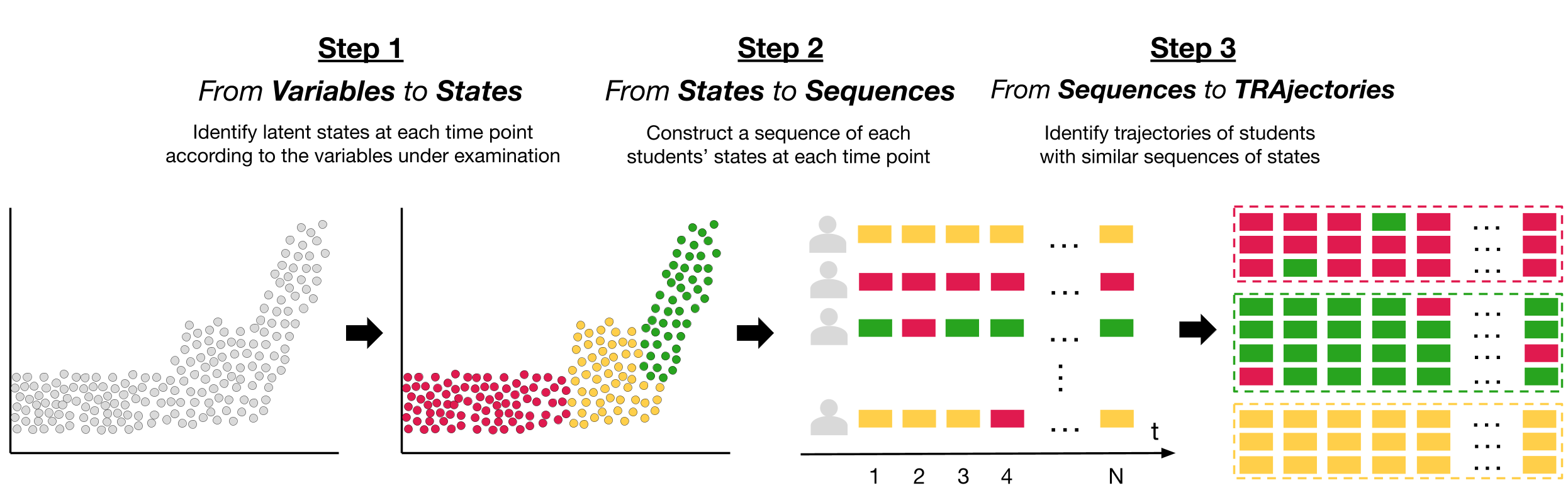
**Figure** 1. Summary of the three steps of the VaSSTra method

Step 1. From variables to states: In the first step of the analysis, we identify the “states” within the data using a method that can capture latent or unobserved patterns from multidimensional data (variables). The said states represent a behavioral pattern, function or a construct that can be inferred from the data. For instance, engagement is a multidimensional construct and is usually captured through several indicators. e.g., students’ frequency and time spent online, course activities, cognitive activities and social interactions. Using an appropriate method, such as person-based clustering in our case, we can derive students’ engagement states for a given activity or course. For instance, the method would classify students who invest significant time, effort and mental work are “engaged.” Similarly, students who are investing low effort and time in studying would be classified as “diseganged.” Such powerful summarization would allow us to use the discretized states in further steps. An important aspect of such states is that they are calculated for a specific timespan. Therefore, in our example we could infer students’ engagement states per activity, per week, per lesson, per course, etc. Sometimes, such time divisions are by design (e.g., lessons or courses), but in other occasions researchers have to establish a time scheme according to the data and research questions (e.g., weeks or days). Computing states for multiple time periods is a necessary step to create time-ordered state sequences and prepare the data for sequence analysis.
Step 2. From states to sequences: Once we have a state for each student at each time point, we can construct an ordered sequence of such states for each student. For example, if we used the scenario mentioned above about measuring engagement states, a sequence of a single student’s engagement states across a six-lesson course would be like the one below. When we convert the ordered states to sequences, we unlock the potential of sequence analysis and life events methods. We are able to plot the distribution of states at each time point, study the individual pathways, the entropy, the mean time spent at each state, etc. We can also estimate how frequently students switch states, and what is the likelihood they finish their sequence in a “desirable” state (i.e., “engaged”).

Step 3. From sequences to trajectories: Our last step is to identify similar trajectories —sequences of states with a similar temporal evolution— using temporal clustering methods (e.g., hidden Markov models or hierarchical clustering). Covariates (i.e., variables that could explain cluster membership) can be added at this stage to help identify why a trajectory has evolved in a certain way. Moreover, sequence analysis can be used to study the different trajectories, and not only the complete cohort. We can compare trajectories according to their sequence properties, or to other variables (e.g., performance).

3 Review of the literature

The VaSSTra method has been used to study different constructs related to students’ learning (Table 11.1), such as engagement [3, 15, 16], roles in computer-supported collaborative learning (CSCL) [17], and learning strategies [18, 19]. Several algorithms have been operationalized to identify latent states from students’ online data. Some examples are: Agglomerative Hierarchical Clustering (AHC) [19], Latent Class Analysis (LCA) [3, 15, 16], Latent Profile Analysis (LPA) [17], and mixture hidden Markov models (MHMM) [18].

Moreover, sequences of states have mostly been used to represent each course in a program [3, 15–18], but also smaller time spans, such as each learning session in a single course [18, 19]. Different algorithms have also been used to cluster sequences of states into trajectories including HMM [3, 19], mixture hidden Markov models (MHMM) [15, 17], and AHC [16, 18]. Moreover, besides the basic aspects of sequence analysis discussed in the previous chapter, previous work have explored advanced features of sequence analysis such as survival analysis [3, 16], entropy [3, 17, 18], sequence implication [3, 18], transitions [3, 17, 18], covariates [17], discriminating subsequences [16] or integrative capacity [17]. Other studies have made used of multi-channel sequence analysis [15, 19], which is covered in Chapter 13 [20].

Table 1. Previous literature in which *VaSSTra* has been used
Ref.	Variables	States	Alphabet	Actor	Time unit	Method Step 1	Method Step 3	Advance sequence methods
[3]	Frequency, time spent and regularity of online activities	Engage- ment	Active, Average, Disengaged, Withdraw	Study program	Course	LCA	HMM	Entropy, sequence implication, survival, transitions
[15]	Frequency, time spent and regularity of online activities. Grades.	Engage- ment, achievement	Active, Average, Disengages. Achiever, Intermediate, Low.	Study program	Course	LCA	MHMM	Multi-channel sequence analysis
[16]	Frequency, time spent and regularity of online activities	Engage- ment	Actively engaged, Averagely engaged, Disengaged, Dropout	Study program	Course	LCA	AHC	Survival analysis, discriminating subsequences, mean time
[17]	Centrality measures	CSCL roles	Influencer, Mediator, Isolate	Study program	Course	LPA	MHMM	Covariate analysis, spell duration, transitions, entropy, integrative capacity
[18]	Online activities	Learning strategies	Diverse, Forum read, Forum interact, Lecture read. Intense diverse, Light diverse, Light interactive, Moderate interactive.	Course. Study program.	Learning session. Course.	MHMM	AHC	Entropy, implication, transitions
[19]	Online activities	Learning strategies	Video-oriented instruction, Slide-oriented instruction, Help-seeking. Assignment struggling, Assignment approaching, Assignment succeeding.	Course	Learning session	AHC	HMM	Multi-channel sequence analysis

4 VassTra with R

In this section we provide a step-by-step tutorial on how to implement VaSSTra with R. To illustrate the method, we will conduct a case study in which we examine students’ engagement throughout all the courses of the first two years of their university studies, using variables derived from their usage of the learning management system.

4.1 The packages

In order to conduct our analysis we will need several packages besides the basic rio (for reading and saving data in different extensions), tidyverse (for data wrangling), cluster (for clustering features), and ggplot2 (for plotting). Below is a brief summary of the rest of the packages needed:

BBmisc: A package with miscellaneous helper functions [21]. We will use its normalize function to normalize our data across courses to remove the differences in students’ engagement that are due to different course implementations (e.g., larger number of learning resources).
tidyLPA: A package for conducting Latent Profile Analysis (LPA) with R [22]. We will use it to cluster students’ variables into distinct clusters or states.
TraMineR: As we have seen in Chapter 10 about sequence analysis [13], this package helps us construct, analyze and visualize sequences from time-ordered states or events [23].
seqhandbook: This package complements TraMineR by providing extra analyses and visualizations [24].
Gmisc: A package with miscellaneous functions for descriptive statistics and plots [25]. We will use it to plot transitions between states.
WeightedCluster: A package for clustering sequences using hierarchical cluster analysis [26]. We will use it to cluster sequences into similar trajectories.

The code below imports all the packages that we need. You might need to install them beforehand using the install.packages command:

library(rio)
library(tidyverse)
library(ggplot2)
library(cluster)
library(BBmisc)
library(tidyLPA)
library(TraMineR)
library(seqhandbook)
library(Gmisc)
library(WeightedCluster)

4.2 The dataset

For our analysis, we will use a dataset of students’ engagement indicators throughout eight courses, corresponding to the first two years of a blended higher education program. The dataset is described in detail in the data chapter. The indicators or variables are calculated from students’ log data in the learning management system, and include the frequency (i.e., number of times) with which certain actions have been performed (e.g., view the course lectures, read forum posts), the time spent in the learning management system, the number of sessions, the number of active days, and the regularity (i.e., consistency and investment in learning). These variables represent students’ bahavioral engagement indicators. The variables are described in detail in Chapter 2 about the datasets of the book [27] and Chapter 7 about predictive learning analytics [28] and in previous works [3]. Below we use rio’s import function to read the data.

LongitudinalData <- 
  import("https://github.com/lamethods/data/raw/main/9_longitudinalEngagement/LongitudinalEngagement.csv")
LongitudinalData

4.3 From variables to states

The first step in our analysis is to detect latent states from the multiple engagement-related variables in our dataset (e.g., frequency of course views, frequency of forum posts, etc.). For this purpose, we will use LPA, a person-based clustering method, to identify each student’s engagement state at each course. We first need to standardize the variables, to account for the possible differences in course implementations (e.g., each course has a different number of learning materials and slightly different duration). This way, the mean value of each indicator will be always 0 regardless of the course. Any value above the mean will be always positive, and any value below will be negative. As such the engagement is measures on the same scale. To standardize the data we first group it by CourseID using tidyverse’s group_by and then we apply the normalize function from the BBmisc package to all the columns that contain the engagement indicators using mutate_at and specifying the range of columns. If we inspect the data now, we will see that all variables are centered around 0.

LongitudinalData |> group_by(CourseID) |>  
  mutate_at(vars(Freq_Course_View:Active_Days), 
            function(x) normalize(x, method = "standardize")) |> 
  ungroup() -> df
df

Now, we need to subset our dataset and choose only the variables that we need for clustering. That is, we exclude the metadata about the user and course, and keep only the variables that we believe are relevant to represent the engagement construct.

to_cluster <- dplyr::select(df, Freq_Course_View, Freq_Forum_Consume, 
                                Freq_Forum_Contribute, Freq_Lecture_View, 
                                Regularity_Course_View, Session_Count, 
                                Total_Duration, Active_Days)

Before we go on, we must choose a seed so we can obtain the same results every time we run the clustering algorithm. We can now finally use tidyLPA to cluster our data. We try from 1 to 10 clusters and different models that enforce different constraints on the data. For example, model 3 takes equal variances and equal covariances, whereas model 6 takes varying variances and varying covariances. You can find out more about this in the tidyLPA documentation [22]. Be aware that running this step may take a while. For more details about LPA, consult the model-based clustering chapter.

set.seed(22294)
Mclustt <- to_cluster |> ungroup() |> 
  single_imputation() |> 
  estimate_profiles(1:10, models = c(1, 2, 3, 6))

Once all the possible cluster models and numbers have been calculated, we can calculate several statistics that will help us choose which is the right model and number of clusters for our data. For this purpose, we use the compare_solutions function from tidyLPA and we use the results of calling this function to plot the BIC and the entropy of each model for the range of cluster numbers that we have tried (1-10). In the model-based clustering chapter you can find out more details about how to choose the best cluster solution.

cluster_statistics <- Mclustt |>  
  compare_solutions(statistics = c("AIC", "BIC","Entropy"))
fits <- cluster_statistics$fits |> mutate(Model = factor(Model))

fits |>
  ggplot(aes(x = Classes,y = Entropy, group = Model, color = Model)) + 
  geom_line() +
  scale_x_continuous(breaks = 0:10) +
   geom_point() +
  theme_minimal() +
  theme(legend.position = "bottom")

fits |>
  ggplot(aes(x = Classes,y = BIC, group = Model, color = Model)) + 
  geom_line() +
  scale_x_continuous(breaks = 0:10) +
  geom_point() +
  theme_minimal() +
  theme(legend.position = "bottom")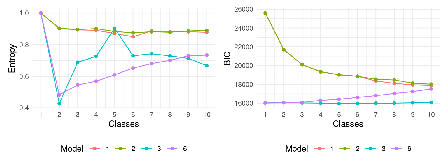

**Figure** 2. Choosing the number of clusters by plotting statistics

Although, based on the BIC values, Model 6 with 3 classes would be the best fit, the entropy for this model is quite low. Instead, Models 1 and 2 have a higher overall entropy and quite a large fall in BIC when increasing from 2 to 3 classes. Taken together, we choose Model 1 with 3 classes which shows better separation of clusters (high entropy) and a large drop in BIC value (elbow). We add the cluster assignment back to the data so we can compare the different variables between clusters and use the cluster assignment for the next steps. Now, for each student’s course enrollment, we have assigned a state (i.e., cluster) that represents the student’s engagement during that particular course.

df$State <- Mclustt$model_1_class_3$model$classification

We can plot the mean variable values for each of the three clusters to understand what each of them represents:

df |> pivot_longer(Freq_Course_View:Active_Days) |> 
  mutate(State = factor(State)) |>
  filter(name %in% names(to_cluster)) |>
  mutate(name = gsub("_", " ", name)) |>
  group_by(name, State) |>
  summarize_if(is.double, mean) -> long_mean

long_mean |>
  ggplot(aes(fill = name, y = value, x = State)) +
  geom_col(position = "dodge") + 
  scale_fill_brewer("", type = "qual", palette=8) +
  theme_minimal() +
  ylab ("Mean value") + 
  theme(legend.position = "bottom")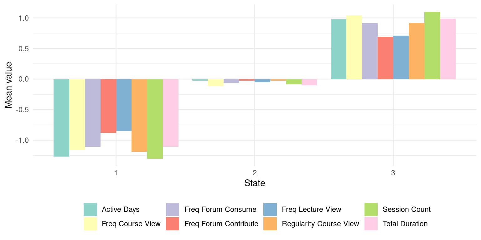

**Figure** 3. Mean value of each variable for each cluster

We clearly see that the first cluster represents students with low mean levels of all engagement indicators; the second cluster represents students with average values, and the third cluster with high values. We can convert the State column of our dataset to a factor to give the clusters an appropriate descriptive label:

engagement_levels = c("Disengaged", "Average", "Active")
df_named <- df |> 
  mutate(State = factor(State, levels = 1:3, labels = engagement_levels))

4.4 From states to sequences

In the previous step, we turned a large amount of variables representing student engagement in a given course into a single state: Disengaged, Average, or Active. Each student has eight engagement states: one per each course (time point in our data) in the first two years of the program. Since the dataset includes the order of each course for each student, we can construct a sequence of the engagement states throughout all courses for each student. To do that we first need to transform our data into a wide format, in which each row represents a single student, and each column represents the student’s engagement state at a given course:

clus_seq_df <- df_named |> arrange(UserID, Sequence) |>
  pivot_wider(id_cols = "UserID", names_from = "Sequence", values_from = "State")

Now we can use TraMineR to construct the sequence and assign colors to represent each of the engagement states:

colors <- c("#28a41f", "#FFDF3C", "#e01a4f")
clus_seq <- seqdef(clus_seq_df , 2:9, 
                   alphabet = sort(engagement_levels), cpal = colors)

We can use the sequence distribution plot from TraMineR to visualize the distribution of each state at each time point (Figure 11.4). We see that the distribution of states is almost constant throughout the eight courses. The ‘Average’ state takes the largest share, followed by the ‘Engaged’ state, and the ‘Disengaged’ state is consistently the least common. For more hints on how to interpret the sequence distribution plot, refer to Chapter 10 [13].

seqdplot(clus_seq, border = NA, use.layout = TRUE, 
         with.legend = T, ncol = 3, legend.prop = 0.2)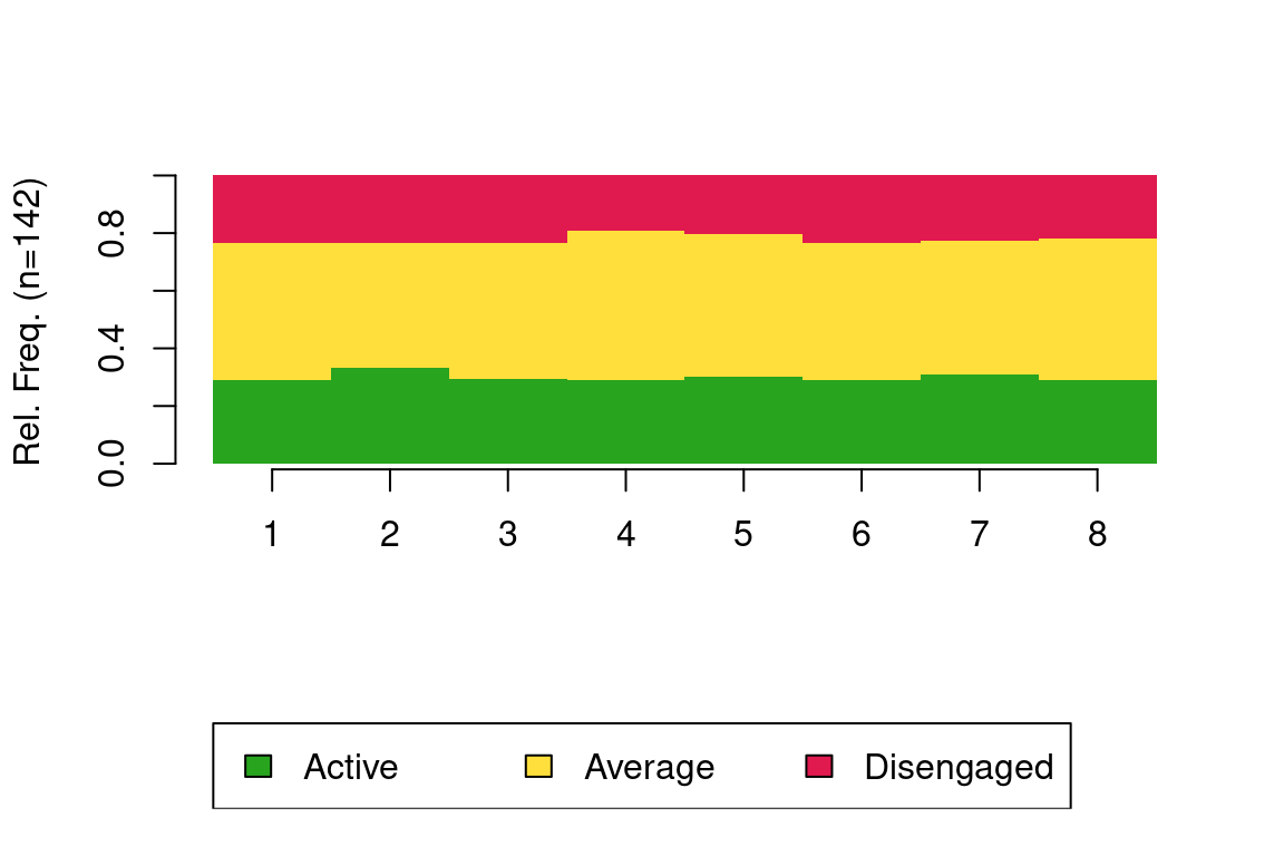

**Figure** 4. Sequence distribution plot of the course states

We can also visualize each of the individual students’ sequences of engagement states using a sequence index plot (Figure 11.5). In this type of visualization, each horizontal bar represents a single student, and each of the eight colored blocks along the bar represents the students’ engagement states. We can order the students’ sequences according to their similarity for a better understanding. To do this, we calculate the substitution cost matrix (seqsubm) and the distance between the sequences according to this cost (seqdist). Then we use an Agglomerative Nesting Hierarchical Clustering algorithm (agnes) to group sequences together according to their similarity (see Chapter 10 [13]). We may now use the seq_heatmap function of seqhandbook to plot the sequences ordered by their similarity. From this plot, we already sense the existence of students that are mostly active, students that are mostly disengaged, and students that are in-between, i.e., mostly average.

sm <- seqsubm(clus_seq, method = "CONSTANT")
mvad.lcss <- seqdist(clus_seq, method = "LCS", sm = sm, with.missing = T)
clusterward2 <- agnes(mvad.lcss, diss = TRUE, method = "ward")
seq_heatmap(clus_seq, clusterward2)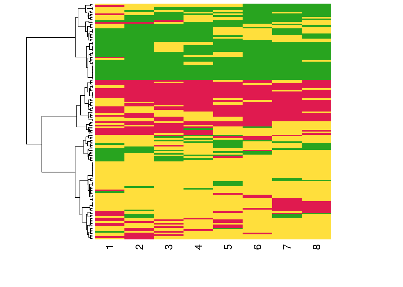

**Figure** 5. Sequence index plot of the course states ordered by sequence distance

4.5 From sequences to trajectories

In the previous step we constructed a sequence of each student’s engagement states throughout eight courses. By plotting these sequences, we observed that there might be distinct trajectories of students that undergo a similar evolution of engagement. In this last step, we use hierarchical clustering to cluster the sequences of engagement states into distinct trajectories of similar engagement patterns. For more details on the clustering technique, please refer to Chapter 8 [29]. To perform hierarchical clustering we first need to calculate the distance between all the sequences. As we have seen in the Sequence Analysis chapter, there are several algorithms to calculate the distance. We choose LCS (Longest Common Subsequence), implemented in the TraMineR package which calculates the distance based on the longest common subsequence.

dissimLCS <- seqdist(clus_seq, method = "LCS")

Now we can perform the hierarchical clustering. For this purpose, we use the hclust function of the stats package

Clustered <- hclust(as.dist(dissimLCS), method = "ward.D2")

We create partitions for clusters ranging from 2 to 10 and we plot the cluster statistics to be able to select the most suitable cluster number.

Clustered_range <- as.clustrange(Clustered, diss = dissimLCS, ncluster = 10)
plot(Clustered_range, stat = "all", norm = "zscoremed", lwd = 2)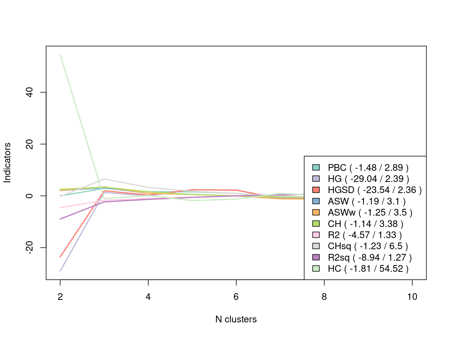

**Figure** 6. Cluster statistics for the hierarchical clustering

There seems to be a maximum for most statistics at three clusters, so we save the cluster assignment for three clusters in a variable named grouping.

grouping <- Clustered_range$clustering$cluster3

Now we can use the variable grouping to plot the sequences for each trajectory using the sequence index plot (Figure 11.7):

seqIplot(clus_seq, group = grouping, sortv = "from.start")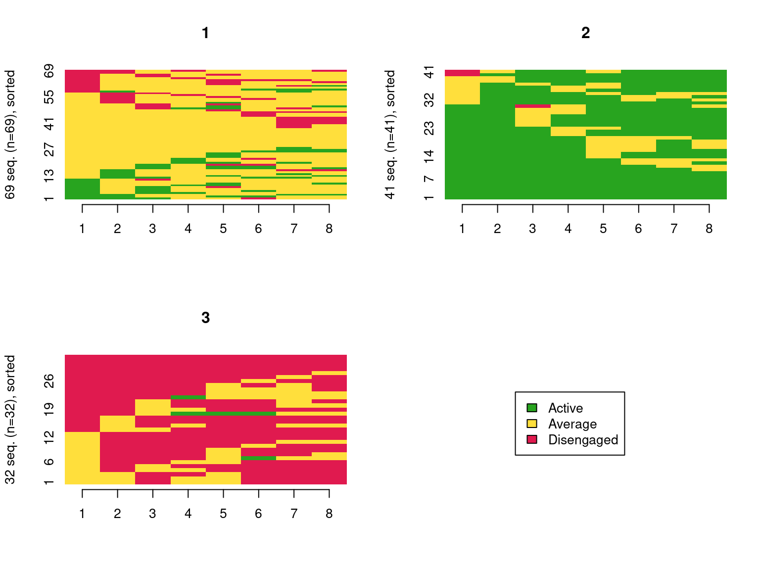

**Figure** 7. Sequence index plot of the course states per trajectory

In Figure 11.7, we see that the first trajectory corresponds to mostly average students, the second one to mostly active students, and the last one to mostly disengaged students. We can rename the clusters accordingly.

trajectories_names = c("Mostly average", "Mostly active", "Mostly disengaged")
trajectories = trajectories_names[grouping]

We can plot the sequence distribution plot to see the overall distribution of the sequences for each trajectory (Figure 11.8).

seqdplot(clus_seq, group = trajectories)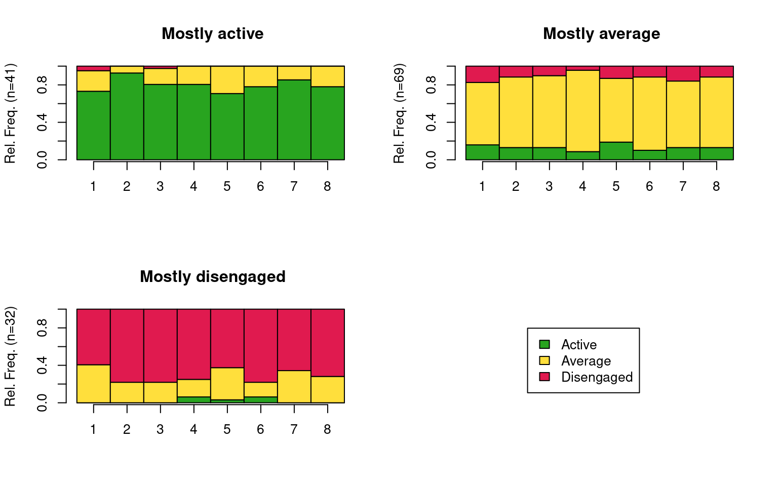

**Figure** 8. Sequence distribution plot of the course states per trajectory

4.6 Studying trajectories

There are many aspects that we can study about our trajectories. For example, we can use the mean time plot to compare the time spent in each engagement state for each trajectory. This plot summarizes the time distribution plot across all time points (Figure 11.9). As expected, we see that the mostly active students spend most of their time in an ‘Active’ state, the mostly average students in an Average state, and the mostly disengaged students in a ‘Disengaged’ state, although they spend quite some time in an ‘Average’ state as well.

seqmtplot(clus_seq, group = trajectories)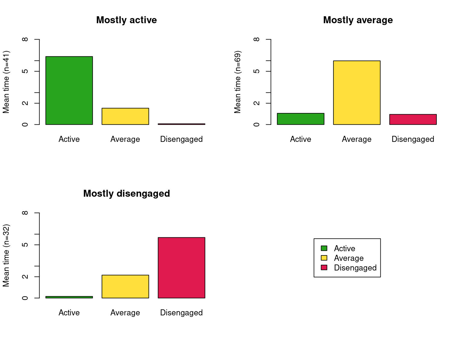

**Figure** 9. Mean time plot of the course states per trajectory

Another very useful plot is the sequence frequency plot (Figure 11.10), that shows the most common sequences in each trajectory and the percentage of all the sequences that they represent. We see that, for each trajectory, the sequence that has all equal engagement states is the most common. The mostly active has, of course, sequences dominated by ‘Active’ states, with sparse average states, and one ‘Disengaged’ state. The mostly disengaged shows a similar pattern dominated by disengaged states with some average and one active state. The mostly average, although it is dominated by ‘Average’ states, shows diversity of shifts to active or disengaged.

seqfplot(clus_seq, group = trajectories)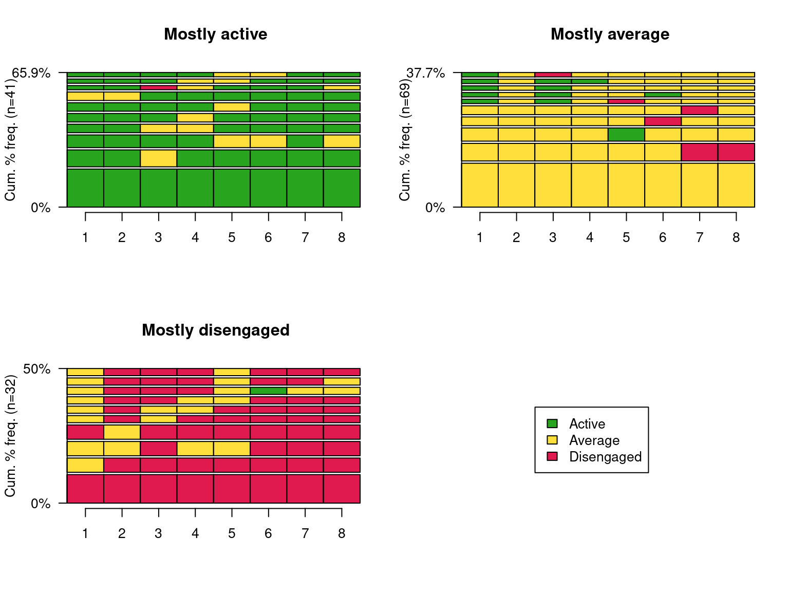

**Figure** 10. The 10 most frequent sequences in each trajectory

To measure the stability of engagement states for each trajectory at each time point, we can use the between-study entropy. Entropy is lowest when all students have the same engagement state at the same time point and highest when the heterogeneity is maximum. We can see that the “Mostly active” and “Mostly disengaged” trajectories have a slightly lower entropy compared to the “Mostly average” one, which is a sign that the students in this trajectory are the least stable (Figure 11.11).

seqHtplot(clus_seq, group = trajectories)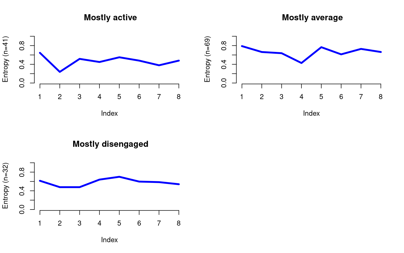

**Figure** 11. Transversal entropy plot of each trajectory

Another interesting aspect to look into is the difference in the most common subsequences among trajectories (Figure 11.12). We first search the most frequent subsequences overall and then compare them among the three trajectories. Interestingly enough, the most frequent subsequence is remaining ‘Active’, and remaining ‘Disengaged’ is number five. Remaining average is not among the top 10 most common subsequences, but rather the subsequences containing the ‘Average’ state always include transitions to other states.

mvad.seqe <- seqecreate(clus_seq)
fsubseq <- seqefsub(mvad.seqe, pmin.support = 0.05, max.k = 2)
discr <- seqecmpgroup(fsubseq, group = trajectories, method = "chisq")
plot(discr[1:10])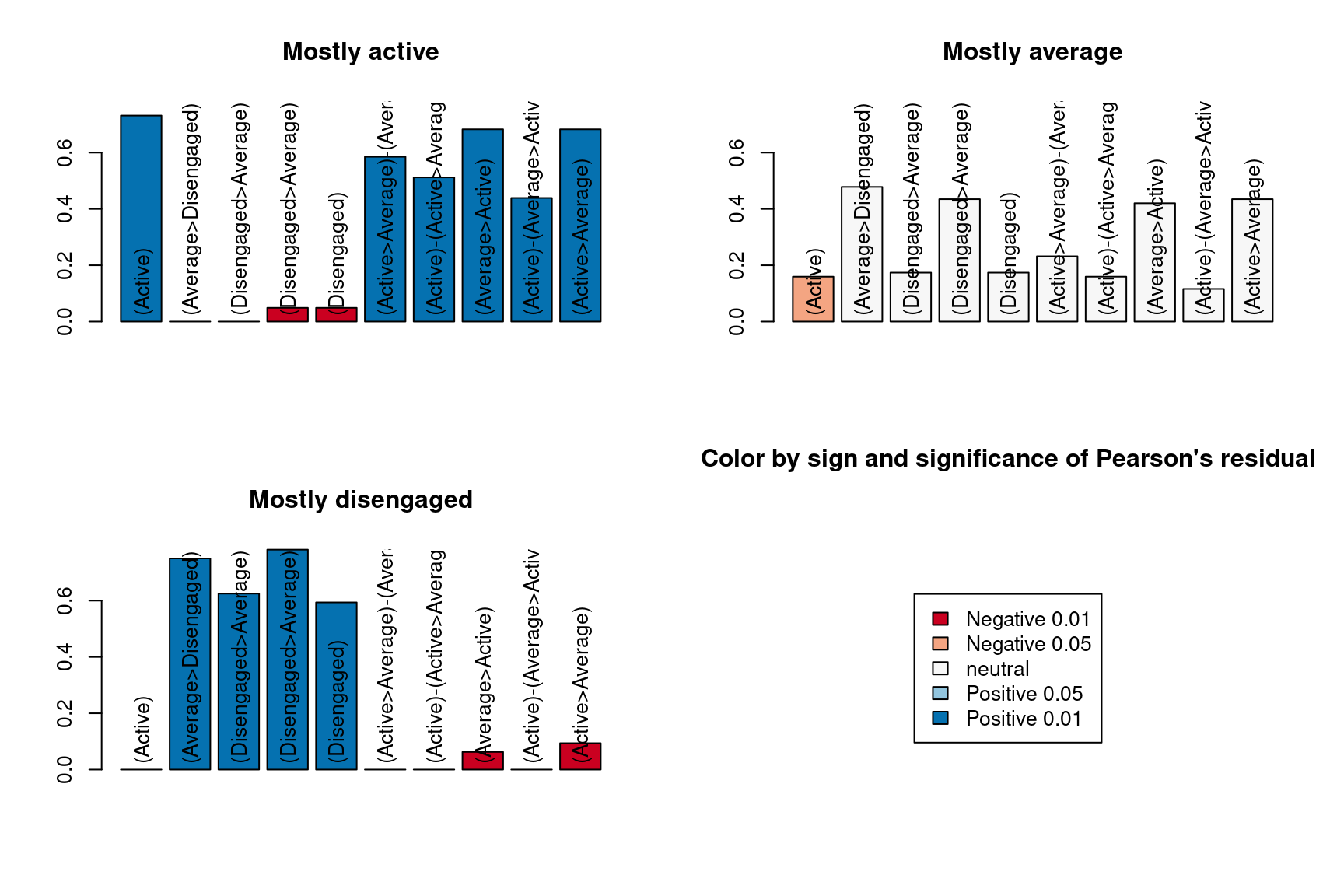

**Figure** 12. Most discriminating subsequences per trajectory

There are other sequence properties that we may need compare among the trajectories. The function seqindic calculates sequence properties for each individual sequence (Table 11.2). Some of these indices need additional information about the sequences, namely, which are the positive and the negative states. In our case, we might consider the Active state to be positive and the Disengaged state to be negative. Below we discuss some of the most relevant measures:

Trans: Number of transitions. It represents the number of times there has been a change of state. If a sequence maintains the same state throughout its whole length, the value of Trans would be zero; if there were two shifts of state, the value would be 2.
Entr: Longitudinal entropy or within-student entropy is a measure of the diversity of the sequence states. In contrast with the transversal or between-students entropy that we saw earlier (Figure 11.11), which is calculated per time point, longitudinal entropy is calculated per sequence (i.e., which represents a student’s engagement through the courses in a program in this case). Longitudinal entropy is calculated using Shannon’s entropy formula. Sequences that remain in the same state most of the time have a low entropy whereas sequences that shift states continuously with great diversity have a high entropy.
Cplx: The complexity index is a composite measure of a sequence’s complexity based on the number of transitions and the longitudinal entropy. It measures the variety of states within a sequence, as well as the frequency and regularity of transitions between them. In other words, a sequence with a high complexity index is characterized by many different and unpredictable states or events, and frequent transitions between them.
Prec: Precarity is a measure of the (negative) stability or predictability of a sequence. It measures the proportion of time that a sequence spends in negative or precarious states, as well as the frequency and duration of transitions between positive and negative states. A sequence with a high precarity index is characterized by a high proportion of time spent in negative or precarious states, and frequent transitions between positive and negative states.
Volat: Objective volatility represents the average between the proportion of states visited and the proportion of transitions (state changes). It is measure of the variability of the states and transitions in a sequence. A sequence with high volatility would be characterized by frequent and abrupt changes in the states or events, while a sequence with low volatility would have more stable and predictable patterns.
Integr: Integrative capacity (potential) is the ability to reach a positive state and then stay in a positive state. Sequences with a high integrative capacity not only include positive states but also manage to stay in such positive states.

Indices <- seqindic(clus_seq,
            indic = c("trans","entr","cplx","prec","volat","integr"), 
            ipos.args = list(pos.states = c("Active")), 
            prec.args = list(c("Disengaged")))

Table 2. Sequence indicators
	Trans	Entr	Volat	Cplx	Integr	Prec
1	2.000	0.343	0.393	0.313	0.000	0.600
2	2.000	0.343	0.393	0.313	0.000	0.600
3	4.000	0.512	0.536	0.541	0.000	0.964
4	0.000	0.000	0.000	0.000	1.000	0.000
5	4.000	0.631	0.536	0.600	0.000	1.159
6..141
142	2.000	0.343	0.393	0.313	0.917	0.006

We can compare the distribution of these indices between the different trajectories to study their different properties (Figure 11.13). Below is an example for precarity and integrative capacity. We clearly see how the Mostly disengaged trajectory has the highest value of precarity, whereas the Mostly active students have the highest integrative capacity. Beyond a mere visual representation, we could also conduct statistical tests to compare whether these properties differ significantly from each other among trajectories.

Indices$Trajectory = trajectories

Indices |> ggplot(aes(x = Trajectory, y = Prec, fill = Trajectory)) + 
  geom_boxplot() + scale_fill_manual(values = colors) + 
  theme_minimal() + theme(legend.position = "none")

Indices |> ggplot(aes(x = Trajectory, y = Integr, fill = Trajectory)) + 
  geom_boxplot() + scale_fill_manual(values = colors) + 
  theme_minimal() + theme(legend.position = "none")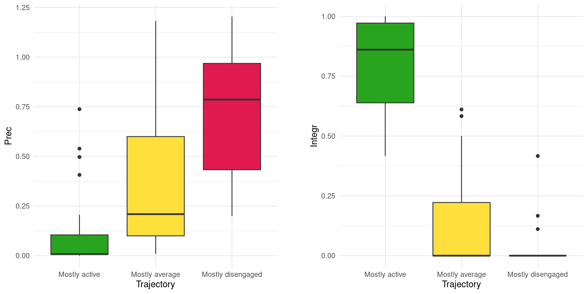

**Figure** 13. Comparison of sequence indicators between trajectories

As we have mentioned, an important aspect of the study of students’ longitudinal evolution is looking at the transitions between states. We can calculate the transitions using seqtrate from TraMineR and plot them using transitionPlot from Gmisc.

transition_matrix = seqtrate(clus_seq, count = T)

From the transition matrix and Figure 11.14 we can see how most transitions are between one state and the same (no change). The most unstable state is ‘Average’ with frequent transitions both to ‘Active’ and ‘Disengaged’. Both ‘Active’ and ‘Disengaged’ had occasional transitions to ‘Average’ but rarely from one another.

transitionPlot(transition_matrix, 
                              fill_start_box = colors,
                              txt_start_clr = "black",
                              cex = 1,
                              box_txt = rev(engagement_levels))

**Figure** 14. Transition plot between states

5 Discussion

In this chapter, the VaSSTra method is presented as a person-centered approach for the longitudinal analysis of complex behavioral constructs over time. In the step-by-step tutorial, we have analyzed students’ engagement states throughout all the courses in the first two years of program. First, we have clustered all the indicators of student engagement into three engagement states using model-based clustering: active, average and disengaged. This step allowed us to summarize eight continuous numerical variables representing students’ online engagement indicators of each course into a single categorical variable (state). Then, we constructed a sequence of engagement states for each student, allowing us to map the temporal evolution of engagement and make use of sequence analysis methods to visualize and investigate such evolution. Lastly, we have clustered students’ sequences of engagement states into three different trajectories: a mostly active trajectory which is dominated by engaged students who are stable throughout time, a mostly average trajectory with averagely engaged students who often transition to engaged or disengaged states, and a mostly disengaged trajectory with inactive students that fail to catch up and remain disengaged most of the program. As such, VaSSTra offers several advantages over the existing longitudinal methods for clustering (such as growth models or longitudinal k-means) which are limited to a single continuous variable [30–32], instead of taking advantage of multiple variables in the data. Through the summarizing power of visualization, VaSSTra is able to represent complex behaviors captured through several variables using a limited number of states. Moreover, through sequence analysis, we can study how the sequences of such states evolve over time and differ from one another, and whether there are distinct trajectories of evolution.

Several literature reviews of longitudinal studies (e.g., [33]) have highlighted the shortcomings of existing research for using variable-centered methods or ignoring the heterogeneity of students’ behavior. Ignoring the longitudinal heterogeneity means mixing trends of different types, e.g., an increasing trend in a subgroup and a decreasing trend in another subgroup exist. Another limitation of the existing longitudinal clustering methods is that cluster membership can not vary with time so one student is assigned to a single longitudinal cluster, which makes it challenging to study variability and transitions.

As we have seen in the literature review section, the VaSSTra method can be adapted to various scenarios beyond engagement, such as collaborative roles, attitudes, achievement, or self-efficacy, and can be used with different time points such as tasks, days, weeks, or school years. The reader should refer to Chapter 8 [29] and Chapter 9 [34] about clustering to learn other clustering techniques that may be more appropriate for transforming different types of variables into states (that is, conducting the first step of VaSSTra). Moreover, in Chapter 10 [13], the basics of sequence analysis are described, including how to cluster sequences into trajectories using different distance measures that might be more appropriate in different situations. The next chapter (Chapter 12) [35] presents Markovian modeling, which constitutes another way of clustering sequences into trajectories according to their state transitions. Lastly, Chapter 13 [20] presents multi-channel sequence analysis, which could be used to extend VaSSTra to study several parallel sequences (of several constructs) at the same time.

References

Henrie CR, Bodily R, Manwaring KC, Graham CR (2015) Exploring intensive longitudinal measures of student engagement in blended learning. The International Review of Research in Open and Distributed Learning 16: https://doi.org/10.19173/irrodl.v16i3.2015

Lazarus G, Song J, Jeronimus BF, Fisher AJ (2023) Delineating discrete generalizable states from intraindividual time series: Towards a science of moments. https://doi.org/10.31234/osf.io/4nxqh

Saqr M, López-Pernas S (2021) The longitudinal trajectories of online engagement over a full program. Comput Educ 175:104325. https://doi.org/10.1016/j.compedu.2021.104325

Winne PH (2020) Construct and consequential validity for learning analytics based on trace data. Computers in Human Behavior 112:106457. https://doi.org/10.1016/j.chb.2020.106457

López-Pernas S, Saqr M (2023) From variables to states to trajectories (VaSSTra): A method for modelling the longitudinal dynamics of learning and behaviour. In: Proceedings of the tenth international conference on technological ecosystems for enhancing multiculturality (TEEM’22). Springer, Salamanca, Spain, pp in press

Genolini C, Falissard B (2010) KmL: K-means for longitudinal data. Comput Stat 25:317–328. https://doi.org/10.1007/s00180-009-0178-4

Nagin DS (2014) Group-based trajectory modeling: An overview. Ann Nutr Metab 65:205–210. https://doi.org/10.1159/000360229

Ram N, Grimm KJ (2009) Growth mixture modeling: A method for identifying differences in longitudinal change among unobserved groups. Int J Behav Dev 33:565–576. https://doi.org/10.1177/0165025409343765

Hougaard P (1999). Lifetime Data Analysis 5:239–264. https://doi.org/10.1023/a:1009672031531

10.

Jackson CH (2011) Multi-state models for panel data: The msm package for r. Journal of Statistical Software 38: https://doi.org/10.18637/jss.v038.i08

11.

McClintock BT, Langrock R, Gimenez O, Cam E, Borchers DL, Glennie R, Patterson TA (2020) Uncovering ecological state dynamics with hidden markov models. Ecology Letters 23:1878–1903. https://doi.org/10.1111/ele.13610

12.

Vogelsmeier LVDE, Vermunt JK, Roover KD (2022) How to explore within-person and between-person measurement model differences in intensive longitudinal data with the r package lmfa. Behavior Research Methods. https://doi.org/10.3758/s13428-022-01898-1

13.

Saqr M, López-Pernas S, Helske S, Durand M, Murphy K, Studer M, Ritschard G (2024) Sequence analysis in education: Principles, technique, and tutorial with r. In: Saqr M, López-Pernas S (eds) Learning analytics methods and tutorials: A practical guide using R. Springer

14.

Jovanović J, Gašević D, Dawson S, Pardo A, Mirriahi N (2017) Learning analytics to unveil learning strategies in a flipped classroom. The Internet and Higher Education 33:74–85. https://doi.org/10.1016/j.iheduc.2017.02.001

15.

Saqr M, López-Pernas S, Helske S, Hrastinski S (2023) The longitudinal association between engagement and achievement varies by time, students’ profiles, and achievement state: A full program study. Comput Educ 199:104787. https://doi.org/10.1016/j.compedu.2023.104787

16.

Saqr M, López-Pernas S (2021) The dire cost of early disengagement: A four-year learning analytics study over a full program. In: Technology-Enhanced learning for a free, safe, and sustainable world. Springer International Publishing, Cham, pp 122–136

17.

Saqr M, López-Pernas S (2022) How CSCL roles emerge, persist, transition, and evolve over time: A four-year longitudinal study. Comput Educ 104581. https://doi.org/10.1016/j.compedu.2022.104581

18.

Saqr M, López-Pernas S, Jovanović J, Gašević D (2023) Intense, turbulent, or wallowing in the mire: A longitudinal study of cross-course online tactics, strategies, and trajectories. internet high 57:100902. https://doi.org/10.1016/j.iheduc.2022.100902

19.

López-Pernas S, Saqr M (2021) Bringing synchrony and clarity to complex multi-channel data: A learning analytics study in programming education. IEEE Access. https://doi.org/10.1109/ACCESS.2021.3134844

20.

López-Pernas S, Saqr M, Helske S, Murphy K (2024) Multichannel sequence analysis in educational research using r. In: Saqr M, López-Pernas S (eds) Learning analytics methods and tutorials: A practical guide using R. Springer, pp in–press

21.

Bischl B, Lang M, Bossek J, Horn D, Richter J, Surmann D (2022) BBmisc: Miscellaneous helper functions for b. bischl

22.

Rosenberg JM, Beymer PN, Anderson DJ, Van Lissa CJ, Schmidt JA (2018) tidyLPA: An r package to easily carry out latent profile analysis (LPA) using open-source or commercial software. Journal of Open Source Software 3:978. https://doi.org/10.21105/joss.00978

23.

Gabadinho A, Ritschard G, Müller NS, Studer M (2011) Analyzing and visualizing state sequences in r with TraMineR. Journal of Statistical Software 40: https://doi.org/10.18637/jss.v040.i04

24.

Robette N (2023) Seqhandbook: Miscellaneous tools for sequence analysis

25.

Gordon M (2023) Gmisc: Descriptive statistics, transition plots, and more

26.

Studer M (2013) WeightedCluster library manual: A practical guide to creating typologies of trajectories in the social sciences with r. LIVES. https://doi.org/10.12682/LIVES.2296-1658.2013.24

27.

López-Pernas S, Saqr M, Conde J, Del-Río-Carazo L (2024) A broad collection of datasets for educational research training and application. In: Saqr M, López-Pernas S (eds) Learning analytics methods and tutorials: A practical guide using R. Springer, pp in–press

28.

Jovanovic J, López-Pernas S, Saqr M (2024) Predictive modelling in learning analytics using R. In: Saqr M, López-Pernas S (eds) Learning analytics methods and tutorials: A practical guide using R. Springer, pp in–press

29.

Murphy K, López-Pernas S, Saqr M (2024) Dissimilarity-based clustering educational data using R. In: Saqr M, López-Pernas S (eds) Learning analytics methods and tutorials: A practical guide using R. Springer, pp in–press

30.

Alhadabi A, Li J (2020) Trajectories of academic achievement in high schools: Growth mixture model. J Educ Issu 6:140. https://doi.org/10.5296/jei.v6i1.16775

31.

Shin S, Rachmatullah A, Ha M, Lee J-K (2018) A longitudinal trajectory of science learning motivation in korean high school students. J Balt Sci Educ 17:674–687. https://doi.org/10.33225/jbse/18.17.674

32.

Vanacore K, Dieter K, Hurwitz L, Studwell J (2021) Longitudinal clusters of online educator portal access: Connecting educator behavior to student outcomes. In: LAK21: 11th international learning analytics and knowledge conference. ACM

33.

Salmela-Aro K, Tang X, Symonds J, Upadyaya K (2021) Student engagement in adolescence: A scoping review of longitudinal studies 2010-2020. J Res Adolesc 31:256–272. https://doi.org/10.1111/jora.12619

34.

Scrucca L, Saqr M, López-Pernas S, Murphy K (2024) An introduction and r tutorial to model-based clustering in education via latent profile analysisg. In: Saqr M, López-Pernas S (eds) Learning analytics methods and tutorials: A practical guide using R. Springer, pp in–press

35.

Helske J, Helske S, Saqr M, López-Pernas S, Murphy K (2024) A modern approach to transition analysis and process mining with markov models: A tutorial with R. In: Saqr M, López-Pernas S (eds) Learning analytics methods and tutorials: A practical guide using R. Springer, pp in–press