kmeans_pp <- function(X, # data
                      K  # number of centroids
                      ) {

  # sample initial centroid from distinct rows of X
  X       <- unique(as.matrix(X))
  new_center_index <- sample(nrow(X), 1)
  centers <- X[new_center_index,, drop=FALSE]

  # let x be all observations not yet chosen as a centroid
  X <- X[-new_center_index,, drop=FALSE]

  if(K >= 2) {
    # loop over remaining centroids
    for(kk in 2:K) {

      # calculate distances from all observations to all already chosen centroids
      distances <- apply(X, 1, function(x) min(sum((x - centers)^2)))

      # sample new centroid with probability proportional to squared Euclidean distance
      probabilities <- distances/sum(distances)
      new_center_index <- sample(nrow(X), 1, prob=probabilities)

      # record the new centroid and remove it for the next iteration
      centers <- rbind(centers, X[new_center_index,, drop=FALSE])
      X <- X[-new_center_index,, drop=FALSE]
    }
  }

  # add random jitter to distinguish non-unique centroids and return
  centers[duplicated(centers)] <- jitter(centers[duplicated(centers)])
  return(centers)
}8 Dissimilarity-based Cluster Analysis of Educational Data: A Comparative Tutorial using R
Abstract
Clustering is a collective term which refers to a broad range of techniques aimed at uncovering patterns and subgroups within data. Interest lies in partitioning heterogeneous data into homogeneous groups, whereby cases within a group are more similar to each other than cases assigned to other groups, without foreknowledge of the group labels. Clustering is also an important component of several exploratory methods, analytical techniques, and modelling approaches and therefore has been practiced for decades in education research. In this context, finding patterns or differences among students enables teachers and researchers to improve their understanding of the diversity of students —and their learning processes— and tailor their supports to different needs. This chapter introduces the theory underpinning dissimilarity-based clustering methods. Then, we focus on some of the most widely-used heuristic dissimilarity-based clustering algorithms; namely, \(K\)-Means, \(K\)-Medoids, and agglomerative hierarchical clustering. The \(K\)-Means clustering algorithm is described including the outline of the arguments of the relevant R functions and the main limitations and practical concerns to be aware of in order to obtain the best performance. We also discuss the related \(K\)-Medoids algorithm and its own associated concerns and function arguments. We later introduce agglomerative hierarchical clustering and the related R functions while outlining various choices available to practitioners and their implications. Methods for choosing the optimal number of clusters are provided, especially criteria that can guide the choice of clustering solution among multiple competing methodologies —with a particular focus on evaluating solutions obtained using different dissimilarity measures— and not only the choice of the number of clusters \(K\) for a given method. All of these issues are demonstrated in detail with a tutorial in R using a real-life educational data set.
1 Introduction
Cluster analysis is a term used to describe a broad range of techniques which have the goal of uncovering groups of observations in a data set. The typical aim of cluster analysis is to categorise observations into groups in such a way that observations within the same group are in some sense more similar to each other, while being relatively dissimilar to those in other groups [1]. In other words, clustering methods uncover group structure in heterogeneous populations by identifying more homogeneous groupings of observations which may represent distinct, meaningful subpopulations. Using machine learning terminology, cluster analysis corresponds to unsupervised learning, whereby groups are identified by relying solely on the intrinsic characteristics (typically dissimilarities), without guidance from unavailable ground truth group labels. Indeed, foreknowledge of the fixed number of groups in a data set is characteristic of supervised learning and the distinct field of classification analysis.
It is important to note that there is no universally applicable definition of what constitutes a cluster [2, 3]. Indeed, in the absence of external information in the form of existing “true” group labels, different clustering methods can reveal different things about the same data. There are many different ways to cluster the same data set, and different methods may yield solutions with different assignments, or even differ in the number of groups they identify. Consequently, we present several cluster analysis algorithms in this chapter; namely, \(K\)-Means [4] in Section 8.3.1, a generalisation thereof, \(K\)-Medoids [5], in Section 8.3.1.2.3, and agglomerative hierarchical clustering [6] in Section 8.3.2. We apply each method in a comparative study in our tutorial using R [7], with applications to a data set about the participants from discussion forum of a massive open online course (MOOC) for teachers.
The clustering methods we review in this chapter are designed to find mutually exclusive, non-overlapping groups in a data set, i.e., they recover a hard partition whereby each observation belongs to one group only. This is in contrast to soft clustering approaches under which each observation is assigned a probability of belonging to each group. One such example of soft clustering is the model-based clustering paradigm, which is discussed in the later Chapter 9 [8]. While model-based clustering methods, as the name suggests, are underpinned by the assumption of generative probabilistic models [9], the more traditional dissimilarity-based methods on which this chapter is focused are purely algorithmic in nature and rely on heuristic criteria regarding the pairwise dissimilarities between objects.
Heuristic clustering algorithms can be further divided into two categories; partitional clustering (e.g., \(K\)-Means and \(K\)-Medoids) and hierarchical (of which we focus on the agglomerative variant). Broadly speaking, partitional clustering methods start with an initial grouping of observations and iteratively update the clustering until the “best” clustering is found, according to some notion of what defines the “best” clustering. Hierarchical clustering methods, on the other hand, is more sequential in nature; a tree-like structure of nested clusterings is built up via successive mergings of similar observations, according to a defined similarity metric. In our theoretical expositions and our applications in the R tutorial, we provide some guidelines both on how to choose certain method-specific settings to yield the best performance and how to determine the optimal clustering among a set of competing methods.
The remainder of this chapter proceeds as follows. In Section 8.2, we review relevant literature in which dissimilarity-based clustering methods have been applied in the realm of educational research. In Section 8.3, we describe the theoretical underpinnings of each method in turn and discuss relevant practical guidelines which should be followed to secure satisfactory performance from each method throughout. Within Section 8.4, we introduce the data set of our case study in Section 8.4.1 and give an overview of some required pre-processing steps in Section 12.4.3, and then present a tutorial using R for each clustering method presented in this chapter in Section 8.4.2, with a specific focus on identifying the optimal clustering solution in Section 8.4.2.4. Finally, we conclude with a discussion and some recommendations for related further readings in Section 8.5, with a particular focus on some limitations of dissimilarity-based clustering which are addressed by other frameworks in the broader field of cluster analysis.
2 Clustering in education: review of the literature
In education, clustering is among the oldest and most common analysis methods, predating the field of learning analytics and educational data mining by several decades. Such early adoption of clustering is due to the immense utility of cluster analysis in helping researchers to find patterns within data, which is a major pursuit of education research [10]. Interest was fueled by the increasing attention to heterogeneity and individual differences among students, their learning processes, and their approaches to learning [11, 12]. Finding such patterns or differences among students allows teachers and researchers to improve their understanding of the diversity of students and tailor their support to different needs [13]. Finding subgroups within cohorts of students is a hallmark of so-called “person-centered methods”, to which clustering belongs [8].
A person-centered approach stands in contrast to the variable-centered methods which consider that most students belong to a coherent homogeneous group with little or negligible differences [14]. Variable-centered methods assume that there is a common average pattern that represents all students, that the studied phenomenon has a common causal mechanism, and that the phenomenon evolves in the same way and results in similar outcomes amongst all students. These assumptions are largely understood to be unrealistic, “demonstrably false, and invalidated by a substantial body of uncontested scientific evidence” [15]. In fact, several analytical problems necessitate clustering, e.g., where opposing patterns exist [16]. For instance, in examining attitudes towards an educational intervention using variable-centered methods, we get an average that is simply the sum of negative and positive attitudes. If the majority of students have a positive attitude towards the proposed intervention —combined with a minority against— the final result will imply that students favour such intervention. The conclusions of this approach are not only wrong but also dangerous as it risks generalising solutions to groups to whom it may cause harm.
Therefore, clustering has become an essential method in all subfields of education (e.g., education psychology, education technology, and learning analytics) having operationalised almost all quantitative data types and been integrated with most of the existing methods [10, 17]. For instance, clustering became an essential step in sequence analysis to discover subsequences of data that can be understood as distinct approaches or strategies of students’ behavior [18]. Similar applications can be found in social network analysis data to identify collaborative roles, or in multimodal data analysis to identify moments of interest (e.g., synchrony). Similarly, clustering has been used with survey data to find attitudinal patterns or learning approaches to mention a few [17]. Furthermore, identifying patterns within students’ data is a prime educational interest in its own right and therefore, has been used extensively as a standalone analysis technique to identify subgroups of students who share similar interests, attitudes, behaviors, or background.
Clustering has been used in education psychology for decades to find patterns within self-reported questionnaire data. Early examples include the work of Beder and Valentine [19] who used responses of a motivational questionnaire to discover subgroups of students with different motivational attitudes. Similarly, Clément et al. [20] used the responses of a questionnaire that assessed anxiety and motivation towards learning English as a second language to find clusters which differentiated students according to their attitudes and motivation. Other examples include the work by Fernandez-Rio et al. [21] who used hierarchical clustering and \(K\)-Means to identify distinct student profiles according to their perception of the class climate. With the digitalisation of educational institutions, authors also sought to identify students profiles using admission data and learning records. For instance, Cahapin et al. [22] used several algorithms such as \(K\)-Means and agglomerative hierarchical clustering to identify patterns in students’ admission data.
The rise of online education opened many opportunities to investigate students’ behavior in learning management systems based on the trace log data that students leave behind them when working on online activities. An example is the work by Saqr et al. [23], who used \(K\)-Means to cluster in-service teachers’ approaches to learning in a MOOC according to their frequency of clicks on the available learning activities. Recently, research has placed a focus on the temporality of students’ activities, rather than the mere count. For this purpose, clustering has been integrated within sequence analysis to find subsequences which represent meaningful patterns of students behavior. For instance, Jovanovic et al. [24] used hierarchical clustering to identify distinct learning sequential patterns based on students’ online activities in a learning management system within a flipped classroom, and found a significant association between the use of certain learning sequences and learning outcomes. Using a similar approach, López-Pernas et al. [25] used hierarchical clustering to identify distinctive learning sequences in students’ use of the learning management system and an automated assessment tool for programming assignments. They also found an association between students’ activity patterns and their performance in the course final exam. Several other examples exist for using clustering to find patterns within sequence data [16, 26, 27].
A growing application of clustering can be seen in the study of computer-supported collaborative learning. Saqr and López-Pernas [28] used cluster analysis to discover students with similar emergent roles based on their forum interaction patterns. Using the \(K\)-Means algorithm and students’ centrality measures in the collaboration network, they identified three roles: influencers, mediators, and isolates. Perera et al. [29] used \(K\)-Means to find distinct groups of similar teams and similar individual participating students according to their contributions in an online learning environment for software engineering education. They found that several clusters which shared some distinct contribution patterns were associated with more positive outcomes. Saqr and López-Pernas [30] analysed the temporal unfolding of students’ contributions to group discussions. They used hierarchical clustering to identify patterns of distinct students’ sequences of interactions that have a similar start and found a relationship between such patterns and student achievement.
An interesting application of clustering in education concerns the use of multimodal data. For instance, Vieira et al. [31] used \(K\)-Means clustering to find patterns in students’ presentation styles according to their voice, position, and posture data. Other innovative uses involve students’ use of educational games [32, 33], virtual reality [34], or artificial intelligence [35]. Though this chapter illustrates traditional dissimilarity-based clustering algorithms with applications using R to data on the centrality measures of the participants of a MOOC, along with related demographic characteristics, readers are also encouraged to read Chapter 9 [8] and Chapter 10 [18] in which further tutorials are presented and additional literature is reviewed, specifically in the contexts of clustering using the model-based clustering paradigm and clustering longitudinal sequence data, respectively. We now turn to an explication of the cluster analysis methodologies used in this chapter’s tutorial.
3 Clustering methodology
In this section, we describe some of the theory underpinning the clustering methods used in the later R tutorial in Section 8.4. We focus on some of the most widely-known heuristic dissimilarity-based clustering algorithms; namely, \(K\)-means, \(K\)-medoids, and agglomerative hierarchical clustering. In Section 8.3.1, we introduce \(K\)-Means clustering by describing the algorithm, outline the arguments to the relevant R function kmeans(), and discuss some of the main limitations and practical concerns researchers should be aware of in order to obtain the best performance when running \(K\)-Means. We also discuss the related \(K\)-Medoids algorithm and the associated function pam() in the cluster library [36] in R, and situate this method in the context of an extension to \(K\)-Means designed to overcome its reliance on squared Euclidean distances. In Section 8.3.2, we introduce agglomerative hierarchical clustering and the related R function hclust(), while outlining various choices available to practitioners and their implications. Though method-specific strategies of choosing the optimal number of clusters \(K\) are provided throughout Section 8.3.1 and Section 8.3.2, we offer a more detailed treatment of this issue in Section 8.3.3, particularly with regard to criteria that can guide the choice of clustering solution among multiple competing methodologies, and not only the choice of the number of clusters \(K\) for a given method.
3.1 \(K\)-Means
\(K\)-means is a widely-used clustering algorithm in learning analytics and indeed data analysis and machine learning more broadly. It is an unsupervised technique that seeks to divide a typically multivariate data set into some pre-specified number of clusters, based on the similarities between observations. More specifically, \(K\)-means aims to partition \(n\) objects \(\mathbf{x}_1,\ldots,\mathbf{x}_n\), each having measurements on \(j=1,\ldots,d\) strictly continuous covariates, into a set of \(K\) groups \(\mathcal{C}=\{C_1,\ldots,C_K\}\), where \(C_k\) is the set of \(n_k\) objects in cluster \(k\) and the number of groups \(K \le n\) is pre-specified by the practitioner and remains fixed. \(K\)-means constructs these partitions in such a way that the squared Euclidean distance between the row vector for observations in a given cluster and the centroid (i.e., mean vector) of the given cluster are smaller than the distances to the centroids of the remaining clusters. In other words, \(K\)-means aims to learn both the cluster centroids and the cluster assignments by minimising the within-cluster sums-of-squares (i.e., variances). Equivalently, this amounts to maximising the between-cluster sums-of-squares, thereby capturing heterogeneity in a data set by partitioning the observations into homogeneous groups. What follows is a brief technical description of the \(K\)-Means algorithm in Section 8.3.1.1, after which we describe some limitations of \(K\)-Means and discuss practical concerns to be aware of in order to optimise the performance of the method in Section 8.3.1.2. In particular, we present the widely-used \(K\)-Medoids extension in Section 8.3.1.2.3.
3.1.1 \(K\)-Means algorithm
The origins of \(K\)-Means are not so straightforward to summarise. The name was initially used by James MacQueen in 1967 [4]. However, the standard algorithm was first proposed by Stuart Lloyd in a Bell Labs technical report in 1957, which was later published as a journal article in 1982 [37]. In order to understand the ideas involved, we must first define some relevant notation. Let \(\mu_k^{(j)}\) denote the centroid value for the \(j\)-th variable in cluster \(C_k\) by \[\mu_k^{(j)} = \frac{1}{n_k}\sum_{\mathbf{x}_i \in C_k} x_{ij}\] and the complete centroid vector for cluster \(C_k\) by \[\boldsymbol{\mu}_k = \left(\mu_k^{(1)}, \ldots, \mu_k^{(p)}\right)^\top.\] These centroids therefore correspond to the arithmetic mean vector of the observations in cluster \(C_k\). Finding both these centroids \(\boldsymbol{\mu}_1,\ldots,\boldsymbol{\mu}_K\) and the clustering partition \(\mathcal{C}\) is computationally challenging and typically proceeds by iteratively alternating between allocating observations to clusters and then updating the centroid vectors. Formally, the objective is to minimise the total within-cluster sum-of-squares \[ \sum_{i=1}^n\sum_{k=1}^K z_{ik} \lVert \mathbf{x}_i - \boldsymbol{\mu}_k\rVert_2^2, \tag{1}\]
where \(\lVert\mathbf{x}_i - \boldsymbol{\mu}_k\rVert_2^2=\sum_{j=1}^p\left(x_{ij}-\mu_k^{(j)}\right)^2\) denotes the squared Euclidean distance to the centroid \(\boldsymbol{\mu}_k\) — such that \(\lVert\cdot\rVert_2\) denotes the \(\ell^2\) norm— and \(\mathbf{z}_i=(z_{i1},\ldots,z_{iK})^\top\) is a latent variable such that \(z_{ik}\) denotes the cluster membership of observation \(i\); \(z_{ik}=1\) if observation \(i\) belongs to cluster \(C_k\) and \(z_{ik}=0\) otherwise. This latent variable construction implies \(\sum_{i=1}^n z_{ik}=n_k\) and \(\sum_{k=1}^Kz_{ik}=1\), such that each observation belongs wholly to one cluster only. As the total variation in the data, which remains fixed, can be written as a sum of the total within-cluster sum-of-squares (TWCSS) from Equation 8.1 and the between-cluster sum-of-squares as follows
\[\sum_{i=1}^n \left(\mathbf{x}_i - \bar{\mathbf{x}}\right)^2=\sum_{i=1}^n\sum_{k=1}^K z_{ik} \lVert \mathbf{x}_i - \boldsymbol{\mu}_k\rVert_2^2 + \sum_{k=1}^Kn_k\lVert\boldsymbol{\mu}_k - \bar{\mathbf{x}}\rVert_2^2,\]
where \(\bar{\mathbf{x}}\) denotes the overall sample mean vector, minimising the TWCSS endeavours to ensure that observations in the same cluster are maximally similar to observations in the same cluster and maximally dissimilar to those in other clusters.
Using the notation just introduced, a generic \(K\)-means algorithm would proceed as follows:
Initialise: Select the number of desired clusters \(K\) and define \(K\) initial centroid vectors \(\boldsymbol{\mu}_1,\ldots,\boldsymbol{\mu}_K\).
Allocate: Find the optimal \(z_{ik}\) values that minimise the objective, holding the \(\mu_k\) values fixed.
Calculate the squared Euclidean distance between each observation and each centroid vector and allocate each object to the cluster corresponding to the initial centroid to which it is closest in terms of squared Euclidean distance. Looking at the objective function in Equation 8.1 closely and examining the contribution of observation \(i\), we need to choose the value of \(\mathbf{z}_i\) which minimises the expression \(\sum_{k=1}^K z_{ik} \lVert \mathbf{x}_i - \boldsymbol{\mu}_k\rVert_2^2\). This is achieved by setting \(z_{ik}=1\) for the value of \(k\) that has smallest \(\lVert \mathbf{x}_i - \boldsymbol{\mu}_k\rVert_2^2\) and setting \(z_{ik^\prime}=0\:\forall\:k^\prime\ne k\) everywhere else.
- Update: Find the optimal \(\boldsymbol{\mu}_k\) values that minimise the objective, holding the \(z_{ik}\) values fixed.
If we re-write the objective function in Equation 8.1 as \[\sum_{i=1}^n\sum_{k=1}^K\sum_{j=1}^p z_{ik} \left(x_{ij}-\mu_k^{(j)}\right)^2,\] we can use the fact that \[\frac{\partial}{\partial \mu_k^{(j)}}\left(x_{ij}-\mu_k^{(j)}\right)^2=-2\left(x_{ij}-\mu_k^{(j)}\right)\] to obtain \[\frac{\partial}{\partial \mu_k^{(j)}}\sum_{i=1}^n\sum_{k=1}^K\sum_{j=1}^p z_{ik} \left(x_{ij}-\mu_k^{(j)}\right)^2=-2\sum_{i=1}^nz_{ik}\left(x_{ij}-\mu_k^{(j)}\right).\] Solving this expression for \(\mu_k^{(j)}\) yields \[\mu_k^{(j)}=\frac{\sum_{i=1}^nz_{ik}x_{ij}}{\sum_{i=1}^nz_{ik}}=\frac{1}{n_k}\sum_{\mathbf{x}_i \in C_k} x_{ij}.\]
- Iterate: One full iteration of the algorithm consists of an allocation step (Step 2) and an update step (Step 3). Steps 2 and 3 are repeated until no objects can be moved between clusters, at which point the algorithm has converged to at least a local minimum of Equation 8.1.
Upon convergence, we obtain not only the estimated partition \(\mathcal{C}=\{C_1,\ldots,C_K\}\), indicating the cluster membership of each observation, but also the estimated cluster centroids \(\boldsymbol{\mu}_1,\ldots,\boldsymbol{\mu}_K\) which act as cluster prototypes, efficiently summarising the characteristics of each cluster. The algorithm just described is just one standard variant of \(K\)-Means. there have been several algorithms proposed for the same objective which derive their names from the author who proposed them; namely MacQueen [4], Lloyd [37], Forgy [38], and Hartigan and Wong [39]. They differ in some subtle ways, particularly with regard to how initial centroids in Step 1 are chosen and whether Steps 3 and 4 are applied to all \(n\) observations simultaneously or whether allocations and centroids are updated for each observation one-by-one (i.e., some variants iterate over Step 2 and Step 3 in a loop over \(i=1,\ldots,n\)). Without going into further details, we note that the default option for kmeans() in R uses the option algorithm="Hartigan-Wong" and this is what we will henceforth adopt throughout.
3.1.2 \(K\)-Means limitations and practical concerns
Though \(K\)-Means is a useful tool in many application contexts due to its conceptual and computational simplicity —so ubiquitous, in fact, that the kmeans() function in R is available without loading any additional libraries— it suffers from numerous limitations and some care is required in order to obtain reasonable results. We now discuss some of the main limitations in turn, but note that each is addressed explicitly throughout the \(K\)-Means application portion of the R tutorial in Section 8.4.2.1. The concerns relate to choosing \(K\) (Section 8.3.1.2.1), choosing initial centroids \(\boldsymbol{\mu}_1,\ldots,\boldsymbol{\mu}_K\) (Section 8.3.1.2.2), and relaxing the reliance on squared Euclidean distances with the more general \(K\)-Medoids method (Section 8.3.1.2.3).
3.1.2.1 Fixed \(K\) and the elbow method
The first major drawback is that the number of clusters \(K\) must be pre-specified. This is a key input parameter: if \(K\) is too low, dissimilar observations will be wrongly grouped together; if \(K\) is too large, observations will be partitioned into many small, similar clusters which may not be meaningfully different. Choosing the optimal \(K\) necessitates running the algorithm at various fixed values of \(K\) and finding the single value of \(K\) which best balances interpretability, parsimony, and fit quality. Fit quality is measured by the TWCSS, i.e., the objective function in Equation 8.1. Increasing \(K\) indefinitely will cause the TWCSS to decrease indefinitely, but this is not what we want. Instead, we seek a \(K\) value beyond which the decrease in TWCSS is minimal, in order to yield a parsimonious solution with a reasonable number of clusters to interpret, without overfitting the data or merely subdividing the actual groups. Thus, a commonly used heuristic graphical method for determining the optimal \(K\) value is to plot a range of \(K\) values against the corresponding obtained TWCSS values and look for an “elbow” or kink in the resulting curve. Such a plot will guide the choice of \(K\) in the \(K\)-Means portion of R tutorial which follows in Section 8.4.2.1.
3.1.2.2 Initialisation and \(K\)-Means
An especially pertinent limitation which must be highlighted is that \(K\)-Means is liable to converge to sub-optimal local minima, i.e., it is not guaranteed to converge to the global minimum of the objective function in Equation 8.1. Many practitioners have observed that the performance of \(K\)-Means is particularly sensitive to a good choice of initial cluster centroids in Step 1. Indeed, as different initial settings can lead to different clusterings of the same data, good starting values are vital to the success of the \(K\)-Means algorithm. Typically, \(K\) random vectors are used to define the initial \(\boldsymbol{\mu}_1,\ldots,\boldsymbol{\mu}_K\) centroids. One means of mitigating (but not completely remedying) the problem is to run \(K\)-Means with a suitably large number of random starting values and choose the solution associated with the set of initial centroids which minimise the TWCSS criterion.
In order to contextualise this issue, it is prudent to first describe some of the main arguments to the kmeans() R function. The following list is a non-exhaustive list of the available arguments to kmeans():
x: a numeric matrix of data or adata.framewith all numeric columns.centers: either the number of clusters \(K\) or a set of \(K\) initial (distinct) cluster centroids.nstart: ifcentersis specified as a number, this represents the number of random sets of \(K\) initial centroids with which to run the algorithm.iter.max: the maximum number of allocation/update cycles allowed per set of initial centroids.
The arguments nstart and iter.max have default values of 1 and 10, respectively. Thus, a user running kmeans() with centers specified as a number will, by default, only use one random set of initial centroids, to which the results are liable to be highly sensitive, and will have the algorithm terminate after just ten iterations, regardless of whether convergence was achieved. It would seem be an improvement, therefore, to increase the values of nstart and iter.max from these defaults. Fortunately, the function automatically returns the single optimal solution according to the random initialisation which yields the lowest TWCSS when nstart exceeds 1.
Though this will generally lead to better results, this approach can be computationally onerous if the number of observations \(n\), number of features \(d\), or size of the range of fixed \(K\) values under consideration is large. An alternative strategy, which greatly reduces the computational burden and the sensitivity of the final solution to the initial choices of \(\boldsymbol{\mu}_1,\ldots,\boldsymbol{\mu}_k\) is to choose a suitable set of informed starting values in a data-driven fashion. To this end, the so-called \(K\)-Means algorithm was proposed [40] in order to improve the performance of \(K\)-Means by replacing Step 1 with an iterative distance-weighting scheme to select the initial cluster centroids. Though there is still randomness inherent in \(K\)-Means, this initialisation technique ensures that the initial centroids are well spread out across the data space, which increases the likelihood of converging to the true global minimum. The \(K\)-Means algorithm works as follows:
Choose an initial centroid uniformly at random from the rows of the data set.
For each observation not yet chosen as a centroid, compute \(D^2(\mathbf{x}_i)\), which represents the squared Euclidean distance between \(\mathbf{x}_i\) and the nearest centroid that has already been chosen.
Randomly sample new observation as a new centroid vector with probability proportional to \(D^2(\mathbf{x}_i)\).
Repeat Steps B and C until \(K\) centroids have been chosen. If any of the chosen initial centroids are not distinct, add a small amount of random jitter to distinguish the non-unique centroids.
Proceed as per Steps 2–4 of the traditional \(K\)-Means algorithm (or one of its variants).
Although these steps take extra time, \(K\)-Means itself tends to converge very quickly thereafter and thus \(K\)-Means actually reduces the computational burden. A manual implementation of the \(K\)-Means is provided by the function kmeans_pp() below. Its output can be used as the centers argument when running kmeans().
However, it should be noted that there is still inherent randomness in \(K\)-Means —note the use of sample() in lines 7 and 22— and the algorithm is liable to produce different initial centroids in different runs on the same data. In effect, \(K\)-Means does not remove the burden of random initialisation; it is merely a way to have more informed random initialisations. Thus, it would be prudent to run \(K\)-Means with \(K\)-Means initialisation and select the solution which minimises the TWCSS, to transfer the burden of requiring multiple runs of \(K\)-Means with random starting values to fewer runs of \(K\)-Means followed by \(K\)-Means with more informed starting values. We adopt this strategy in the later R tutorial in Section 8.4.2.1.
3.1.2.3 \(K\)-Medoids and other distances
The \(K\)-Means objective function in Equation 8.1 explicitly relies on squared Euclidean distances and requires all features in the data set to be strictly continuous. An artefact of this distance measure is that it is generally recommended to standardise all features of have a mean of zero and unit variance prior to running \(K\)-Means. In general, standardisation is advisable if the values are of incomparable units (e.g., height in inches and weight in kilogram). More specifically for \(K\)-Means, it is desirable to ensure all features have comparable variances to avoid having variables with higher magnitudes and variances dominate the distance calculation and have an undue prominence on the clustering partition obtained. While we employ such normalisation to the data used in our R tutorial when applying some pre-processing steps in Section 12.4.3, we note that this is not sufficient to overcome all shortcomings of relying on squared Euclidean distances.
For these reasons and more, \(K\)-Medoids —otherwise known as partitioning around medoids (PAM)— was proposed as an extension to \(K\)-Means which allows using any alternative dissimilarity measure [5]. The \(K\)-Medoids objective function is given by \[\sum_{i=1}^n\sum_{k=1}^K z_{ik} d\left(\mathbf{x}_i, \boldsymbol{\psi}_k\right),\] where \(d\left(\mathbf{x}_i, \boldsymbol{\psi}_k\right)\) can be any distance measure rather than squared Euclidean and \(\boldsymbol{\psi}_k\) is used in place of the mean vector \(\boldsymbol{\mu}_k\). The PAM algorithm works in much the same fashion as \(K\)-Means, alternating between an allocation step which assigns each observation to the cluster with the closest \(\boldsymbol{\psi}_k\) (according to the specified distance measure) and an update step which minimises the within-cluster total distance (WCTD). Notably, when minimising with respect to \(\boldsymbol{\psi}_k\), the notion of a cluster centroid \(\boldsymbol{\mu}_k\) is redefined as a cluster medoid \(\boldsymbol{\psi}_k\), which is selected among the rows of the observed data set, i.e., the medoid is the observation \(\mathbf{x}_i\) from which the distance to all other observations currently allocated to the same cluster, according to the specified distance measure, is minimised. Similar to \(K\)-Means, the medoids obtained at convergence again enable straightforward characterisation of a “typical” observation from each cluster and the elbow method from Section 8.3.1.2.1 can be adapted to guide the choice of \(K\) in \(K\)-Medoids by plotting a range of candidate \(K\) values against the within-cluster total distance.
This reformulation has three main advantages. Firstly, the distance \(d\left(\mathbf{x}_i, \boldsymbol{\psi}_k\right)\) is not squared, which diminishes the influence of outliers. As \(K\)-Means relies on squared Euclidean distances, which inflates the distances of atypical observations, and defines centroids as means, it is not robust to outliers. Secondly, by defining the medoids as observed rows of the data, rather than finding the value of \(\boldsymbol{\psi}_k\) that minimises in general, which could potentially be difficult to estimate for complex data types or particularly sophisticated dissimilarity measures, the algorithm can be much more computationally efficient. It requires only a pre-calculated pairwise dissimilarity matrix as input. Finally, the flexibility afforded by being able to modify the dissimilarity measure enables data which are not strictly continuous to be clustered. In other words, \(K\)-Medoids is applicable in cases where the mean is undefined. As examples, one could use the Manhattan or general Minkowski distances as alternatives for clustering continuous data, the Hamming [41], Jaccard [42], or Sørensen-Dice [43, 44] distances for clustering binary data, or the Gower distance [45] for clustering mixed-type data with both continuous and categorical features. The closely related \(K\)-Modes algorithm [46] has also been proposed specifically for purely categorical data applications, as well as the \(K\)-Prototypes algorithm [47] for mixed-type variables applications; neither will considered further in this chapter). As their names suggest, they again redefine the notion of a centroid but otherwise proceed much like \(K\)-Means and \(K\)-Medoids.
The function pam() in the cluster library in R provides an implementation of \(K\)-Medoids, with options for implementing many recent additional speed improvements and improved initialisation strategies [48]. We will discuss these in the \(K\)-Medoids portion of the later R tutorial in Section 8.4.2.2. Most dissimilarity measures we will use are implement in the base-R function dist(), with the exception of the Gower distance which is implemented in the daisy() function in the cluster library.
3.2 Agglomerative hierarchical clustering
Hierarchical clustering is another versatile and widely-used dissimilarity-based clustering paradigm. Though also dissimilarity-based, hierarchical clustering differs from partitional clustering methods like \(K\)-Means and \(K\)-Medoids in that it typically doesn’t avail of the notion of computing distances to a central prototype, be that a centroid mean vector or a medoid, but instead greedily builds a hierarchy of clusters based on dissimilarities between observations themselves and sets of observations. Consequently, a hierarchical clustering solution provides a set of partitions, from a single cluster to as many clusters as observations, rather than the single partition obtained by \(K\)-Means and \(K\)-Medoids. The results of a hierarchical clustering are usually presented in the form of a dendrogram visualisation, which illustrates the arrangement of the set of partitions visited and can help guide the decision of the optimal single clustering partition to extract. However, hierarchical clustering shares some of the advantages \(K\)-Medoids has over \(K\)-Means. Firstly, any valid measure of distance can be used, so it is not restricted to squared Euclidean distances and not restricted to clustering purely continuous data. Secondly, hierarchical clustering algorithms do not require the data set itself as input; all that is required is a matrix of pairwise distances.
Broadly speaking, there are two categories of hierarchical clustering:
Agglomerative: Starting from the bottom of the hierarchy, begin with each observation in a cluster of its own and successively merged pairs of clusters while moving up the hierarchy, until all observations are in one cluster. This approach is sometimes referred to as agglomerative nesting (AGNES; [6]).
Divisive: Starting from the top of the hierarchy, with all observations in one cluster, recursively split clusters while moving down the hierarchy, until all observations are in a cluster of their own. This approach is sometimes referred to as divisive analysis (DIANA; [49]).
However, divisive clustering algorithms such as DIANA are much more computationally onerous for even moderately large data sets. Thus, we focus here on the agglomerative variant of hierarchical clustering, AGNES, which is is implemented in both the agnes() function in the cluster library and the hclust() function in base R. We adopt the latter in the hierarchical clustering portion of the R tutorial in Section 8.4.2.3. That being said, even agglomerative hierarchical clustering has significant computation and memory burdens when \(n\) is large [50, 51].
There are three key decisions practitioners must make when employing agglomerative hierarchical clustering. The first of these, the distance measure, has already been discussed in the context of \(K\)-Medoids. We now discuss the other two in turn; namely, the so-called linkage criterion for quantifying the distances between merged clusters as the algorithm moves up the hierarchy, and the criterion used for cutting the resulting dendrogram to produce a single partition.
3.2.1 Linkage criteria
Agglomerative hierarchical clustering employs two different notions of dissimilarity. There is the distance measure, \(d\), such as Euclidean, Manhattan, or Gower distance, which is used to quantify the distance between pairs of single observations in the data set. Different choices of distance measure can lead to markedly different clustering results and it is thus common to run the hierarchical clustering algorithm with different choices of distance measure and compare the results. However, in the agglomerative setting, individual observations are successively merged into clusters. In order to decide which clusters should be combined, it is necessary to quantify the dissimilarity of sets of observations as a function of the pairwise distances of observations in the sets. This gives rise to the notion of a linkage criterion. At each step, the two clusters separated by the shortest distance are combined; the linkage criteria is precisely the definition of ‘shortest distance’ which differentiates different agglomerative approaches. Again, the choice of linkage criterion can have a substantial impact on the result of the clustering so multiple solutions with different combinations of distance measure and linkage criterion should be evaluated.
There are a number of commonly-used linkage criteria which we now describe. A non-exhaustive list of such linkages follows —only those which we use in the later R tutorial in Section 8.4— in which we let \(\mathcal{A}\) and \(\mathcal{B}\) denote two sets of observations, \(\lvert\cdot\rvert\) denote the cardinality of a set, and \(d(a, b)\) denote the distance between observations in those corresponding sets according to the chosen distance measure. We note that ties for the maximum or minimum distances for complete linkage and single linkage, respectively, are broken at random.
Complete linkage: Define the dissimilarity between two clusters as the distance between the two elements (one in each cluster) which are furthest away from each other according to the chosen distance measure \(d\): \[\max_{a \in \mathcal{A}, b \in \mathcal{B}} d(a, b).\]
Single linkage: Define the dissimilarity between two clusters as the distance between the two elements (one in each cluster) which are closest to each other according to the chosen distance measure \(d\): \[\min_{a \in \mathcal{A}, b \in \mathcal{B}} d(a, b).\]
Average linkage: Define the dissimilarity between two clusters as the average distance according to the chosen distance measure \(d\) between all pairs of elements (on in each cluster): \[\frac{1}{\lvert\mathcal{A}\rvert \times \lvert\mathcal{B}\rvert}\sum_{a \in \mathcal{A}}\sum_{b \in \mathcal{B}}d_(a, b).\]
Centroid linkage: Define the dissimilarity between two clusters \(\mathcal{A}\) and \(\mathcal{B}\) as the distance, according to the chosen distance measure \(d\), between their corresponding centroid vectors \(\boldsymbol{\mu}_{\mathcal{A}}\) and \(\boldsymbol{\mu}_{\mathcal{B}}\): \[d(\boldsymbol{\mu}_{\mathcal{A}}, \boldsymbol{\mu}_{\mathcal{B}}).\]
Ward linkage [52]: Instead of measuring the dissimilarity between clusters directly, define the dissimilarity as the cost of merging two clusters as the increase in total within-cluster variance after merging. In other words, minimise the total within-cluster sum-of-squares by finding the pair of clusters at each step which leads to minimum increase in total within-cluster variance after merging, where \(\mathcal{A} \cup \mathcal{B}\) denotes the cluster obtained after merging, with corresponding centroid \(\boldsymbol{\mu}_{\mathcal{A}\cup\mathcal{B}}\): \[\frac{\lvert\mathcal{A}\rvert \times \lvert \mathcal{B}}{\lvert \mathcal{A} \cup \mathcal{B}\rvert}\lVert\boldsymbol{\mu}_{\mathcal{A}} - \boldsymbol{\mu}_{\mathcal{B}}\rVert_2^2 = \sum_{x\in \mathcal{A}\cup\mathcal{B}}\lVert x - \boldsymbol{\mu}_{\mathcal{A}\cup\mathcal{B}}\rVert_2^2 - \sum_{x \in \mathcal{A}}\lVert x - \boldsymbol{\mu}_{\mathcal{A}}\rVert_2^2 - \sum_{x \in \mathcal{B}}\lVert x - \boldsymbol{\mu}_{\mathcal{B}}\rVert_2^2.\]
The Ward and centroid linkage criteria differ from the other linkage criteria in that they are typically meant to be used only when the initial pairwise distances between observations are squared Euclidean distances. All of the above linkage criteria are implemented in the function hclust(), which is available in R without requiring any add-on libraries to be loaded and specifically performs agglomerative hierarchical clustering. Its main arguments are d, a pre-computed pairwise dissimilarity matrix (as can be created from the function dist()), and method, which specifies the linkage criterion (e.g., "complete", "single", "average", and "centroid"). Special care must be taken when employing Ward’s linkage criterion as two options are available: "ward.D", which assumes that the initial pairwise distance matrix already consists of squared Euclidean distances, and "ward.D2", which assumes the distances are merely Euclidean distances and performs the squaring internally [53].
3.2.2 Cutting the dendrogram
One might notice that when calling hclust(), the number of clusters \(K\) is not specified in advance, as it is when calling kmeans() or pam(). Instead, hclust() returns an object which describes the hierarchy of the tree produced by the clustering process. A visualisation of such a tree is referred to as a dendrogram, which can be thought of as a representation of a set of candidate partitions. In a dendrogram representation of an agglomerative hierarchical clustering solution, each observation is initially in a singleton cluster on its own, along the x-axis, according to their similarities. Thereafter, each observation, and subsequently each set of observations, are merged along the y-axis in a nested fashion. The scale along the y-axis is proportional to the distance, according to the chosen linkage criterion, at which two clusters are combined. In the end, the groups formed towards the bottom of the graph are close together, whereas those at the top of the graph are far apart.
Obtaining a single hard partition of objects into disjoint clusters is obtained by cutting the dendrogram horizontally at the corresponding height. In other words, observations are allocated to clusters by cutting the tree at an appropriate height. Generally, the lower this height, the greater the number of clusters (theoretically, there can be as many clusters as there are observations, \(n\)), while the greater the height, the lower the number of clusters (theoretically, there can be as few as only one cluster, corresponding to no group structure in the data). Thus, an advantage of hierarchical clustering is that the user need not know \(K\) in advance; the user can manually select \(K\) after the fact by examining the constructed tree and fine-tuning the output to find clusters with a desired level of granularity. There is no universally applicable rule for determining the optimal height at which to cut the tree, but it is common to select a height in the region where there is the largest gap between merges, i.e., where there is a relatively wide range of distances over which the number of clusters in the resulting partition does not change. This is, of course, very much guided by the visualisation itself.
In R, one can visualise the dendrogram associated with a particular choice of distance measure and linkage criterion by calling plot() on the output from hclust(). Thereafter, the function cutree() can be used to obtain a single partition. This function takes the arguments tree, which is the result of a call to hclust(), h which is the height at which the tree should be cut, and k which more directly allows the desired number of clusters to be produced. Specifying k finds the corresponding height which yields k clusters and overrides the specification of h.
However, it is often the case that certain combinations of dissimilarity measure and linkage criterion produce undesirable dendrograms. In particular, complete linkage is known to perform poorly in the presence of outliers, given its reliance on maximum distances, and single linkage is known to produce a “chaining” effect on the resulting dendrogram, whereby, due to its reliance on minimum distances, observations tend to continuously join increasingly larger, existing clusters rather than being merged with other observations to form new clusters. A negative consequence of this phenomenon is lack of cohesion: observations at opposite ends of the same cluster in a dendrogram could be quite dissimilar. These limitations can also be attributed to hierarchical clustering —regardless of the linkage employed— optimising a local criterion for each merge, unlike \(K\)-Means and \(K\)-Medoids which endeavour to optimise global objectives.
3.3 Choosing the number of clusters
Determining the number of clusters in a data set is a fraught task. Throughout Section 8.3.1 and Section 8.3.2, method-specific strategies for guiding the choice of \(K\) were presented. However, they are not without their limitations. For \(K\)-Means and \(K\)-Medoids, the elbow method is somewhat subjective and unreliable. Often, the presence of an elbow is not so clear at a single value of \(K\). Likewise, for agglomerative hierarchical clustering, choosing a height at which to cut the dendrogram as the criterion for choosing \(K\) has also been criticised as an overly subjective method. Moreover, these strategies are only capable of identifying the best \(K\) value conditional on the chosen method and do not help to identify the overall best solution among multiple competing methods. Moreover, we are required to choose more than just the optimal \(K\) value when using \(K\)-Medoids (for which different solutions with different dissimilarity measures and different \(K\) values can be obtained) and agglomerative hierarchical clustering (for which different solutions can be obtained using different dissimilarity measures and linkage criteria).
Overcoming these ambiguities and identifying a more general strategy for comparing the quality of clustering partitions is a difficult task for which many criteria have been proposed. Broadly speaking, cluster quality measures fall into two categories:
Comparing of the uncovered partition to a reference clustering (or known grouping labels).
Measuring of internal cluster consistency without reference to ground truth labels.
The first is typically conducted using the Rand index [54] or adjusted Rand index [55], which measure the agreement between two sets of partitions. However, as we will be exploring clustering in exploratory, unsupervised settings, using data for which there is no assumed “true” group structure, we will instead focus on a quality measure of the latter kind. As previously stated, a large number of such criteria have been proposed in the literature: several are summarised in Table 7 of Chapter 10 of this book [18], where they are used to guide the choice of \(K\) for agglomerative hierarchical clustering in the context of sequence analysis. Here, however, for the sake of brevity, we describe only one commonly used criterion which we later employ in the R tutorial in Section 8.4 —which is itself a dissimilarity-based measure and is thus universally applicable to all clustering algorithms we employ— even if in most applications it would be wise to inform the choice of \(K\) with several such quantitative criteria. Moreover, the practitioner’s own subject matter expertise and assessment of the interpretability of the obtained clusters should also be used to inform the choice of \(K\).
The quantitative criterion we employ is referred to as the average silhouette width (ASW) criterion [56], which is routinely used to assess the cohesion and separation of the clusters uncovered by dissimilarity-based methods. Cohesion refers to the tendency to group similar objects together and separation refers to the tendency to group dissimilar objects apart in non-overlapping clusters. As the name implies, the ASW is computed as the average of observation-specific silhouette widths. Under the assumption that \(K>1\), silhouette widths and the ASW criterion are calculated as follows:
Let \(a(i)\) be the average dissimilarity from observation \(i\) to the other members of the same cluster to which observation \(i\) is assigned.
Compute the average dissimilarity from observation \(i\) to the members of all \(K-1\) other clusters: let \(b(i)\) be the minimum such distance computed.
The silhouette for observation \(i\) is then defined to be \[\begin{align*} s(i) &= \frac{b(i) - a(i)}{\max\{a(i), b(i)\}}\\ &= \begin{cases} 1 - \frac{a(i)}{b(i)} & \mbox{if}\:a(i) < b(i)\\ 0& \mbox{if}\:a(i)=b(i)\\ \frac{b(i)}{a(i)} - 1 & \mbox{if}\:a(i) > b(i), \end{cases} \end{align*}\] unless observation \(i\) is assigned to a cluster of size \(1\), in which case \(s(i)=0\). Notably, \(a(i)\) and \(b(i)\) need not be calculated using the same dissimilarity measure with which the data were clustered; it is common to adopt the Euclidean distance.
Define the ASW for a given partition \(\mathcal{C}\) as: \(\mbox{ASW}\left(\mathcal{C}\right)=\frac{1}{n}\sum_{i=1}^n s_i.\)
Given that \(-1 \le s(i) \le 1\), the interpretation of \(s(i)\) is that a silhouette close to \(1\) indicates that the observation has been well-clustered, a silhouette close to \(-1\) indicates that the observation would be more appropriately assigned to another cluster, and a silhouette close to zero indicates that the observation lies on the boundary of two natural clusters. If most values of \(s(i)\) are high, then the clustering solution can be deemed appropriate. This occurs when \(a(i) \ll b(i)\), meaning that observation \(i\) must be well-matched its own cluster and poorly-matched to all other clusters. Conversely, if most \(s(i)\) values are low or even negative, this provides evidence that \(K\) may be too low or too high.
The values of \(s(i)\) can be averaged over all observations assigned to the same cluster, as a measure of how tightly grouped the observations in the given cluster are. The ASW criterion itself is simply the mean silhouette width over all observations in the entire data set. Generally, clustering solutions with higher ASW are to be preferred, however it is also prudent to dismiss solutions with many negative silhouettes or particularly low cluster-specific mean silhouettes. A silhouette plot can help in this regard; such a plot depicts all values of \(s(i)\), grouped according to the corresponding cluster and in decreasing order within a cluster. In the R tutorial which follows, ASW values and silhouette plots will guide the choice of an optimal clustering solution in a comparison of multiple methods in Section 8.4.2.4.
4 Tutorial with R
In this section, we will learn how to perform clustering using the R programming language [7], using all methods described throughout Section 8.3. We start by loading the necessary libraries. We will use cluster [36] chiefly for functions related to \(K\)-Medoids and silhouettes. As per other chapters in this book, we use tidyverse [57] for data manipulation and rio [58] for downloading the data: see Section 12.4.3 for details the on the data pre-processing steps employed.
library(cluster)
library(rio)
library(tidyverse)
We note that hierarchical clustering and \(K\)-Means are implemented in base R and thus no dedicated libraries need to be loaded.
4.1 The data set
Our case study will be to identify different groups of participants that have a similar role in the discussion forum of a massive open online course (MOOC) for teachers. For that purpose, we will rely on the centrality measures of the participants which indicate their number of contributions (OutDegree), replies (InDegree), position in the network (Closeness_total), worth of their connections (Eigen), spread of their ideas (Diffusion_degree), and more. For more details about the data set, please refer to the data chapter of the book (Chapter 2; [59]). To learn more about centrality measures and how to calculate them, refer to the social network analysis chapter (Chapter 15; [60]). We will henceforth refer to these data as “the MOOC centralities data set”. We can download and preview the data with the following commands:
URL <- "https://github.com/lamethods/data/raw/main/6_snaMOOC/"
df <- import(paste0(URL, "Centralities.csv"))
df
Additionally, a number of categorical variables pertaining to demographic characteristics are available for the same participants. Again, please refer to the data chapter of the book (Chapter 2; [59]) for more details on these variables. With an appropriate distance measure, namely the Gower distance measure, we will incorporate some of these variables in our applications of \(K\)-Medoids and agglomerative hierarchical clustering (but not \(K\)-Means) in addition to the continuous variables contained in df, largely for the purpose of demonstrating clustering methods which are capable of clustering variables of mixed type. We can download and preview the auxiliary categorical data set with the commands below. Note that we select only the following variables:
experience(coded as a level of experience, 1–3),gender(female or male),region(Midwest, Northeast, South, and West U.S.A., along with International),
for the sake of simplifying the demonstration of mixed-type variables clustering and reducing the computational burden. We also extract the UID column, a user ID which corresponds to the name column in df, which will be required for later merging these two data sets. We also ensure that all but this leading UID column is formatted as a factor.
demog <- import(paste0(URL, "DLT1%20Nodes.csv"))
demog <- demog |>
  select(UID, experience, gender, region) |>
  mutate_at(vars(-UID), as.factor)
demog
4.1.1 Pre-processing the data
In df, the first column (name) is the student identifier, and the remaining columns are each of the centrality measures calculated from students’ interactions in the MOOC forum. We will eventually discard the name column from future analyses; we retain it for the time being so that df and demog can be merged appropriately. The data also contain a small number of observations —only three rows of df— with missing values for the variable Closeness_total, as seen by
df |> is.na() |> which(arr.ind=TRUE) row col
441 441 4
442 442 4
443 443 4Given that none of the clustering methods described in this chapter are capable of accommodating missing data, we remove these three observations for future analyses too. Furthermore, one of the rows in demog has NULL recorded for the gender variable. We remove all invalid rows from both df and demog. The function complete.cases() constructs a completely observed data set by extracting the rows which contain one or more missing values and we augment the index of fully observed rows with an index of non-NULL gender values. Finally, we drop the redundant NULL level from the factor variable gender.
obs_ind <- complete.cases(df) & demog$gender != "NULL"
df$name[!obs_ind] # indices of observations with missing values
[1] 439 441 442 443df <- df |> filter(obs_ind)
demog <- demog |> filter(obs_ind) |> droplevels()Before proceeding any further, it would be prudent to explore the complete data visually, which we do via the matrix of pairwise scatter plots, excluding the name column, in Figure 8.1:
pairs(df[,-1])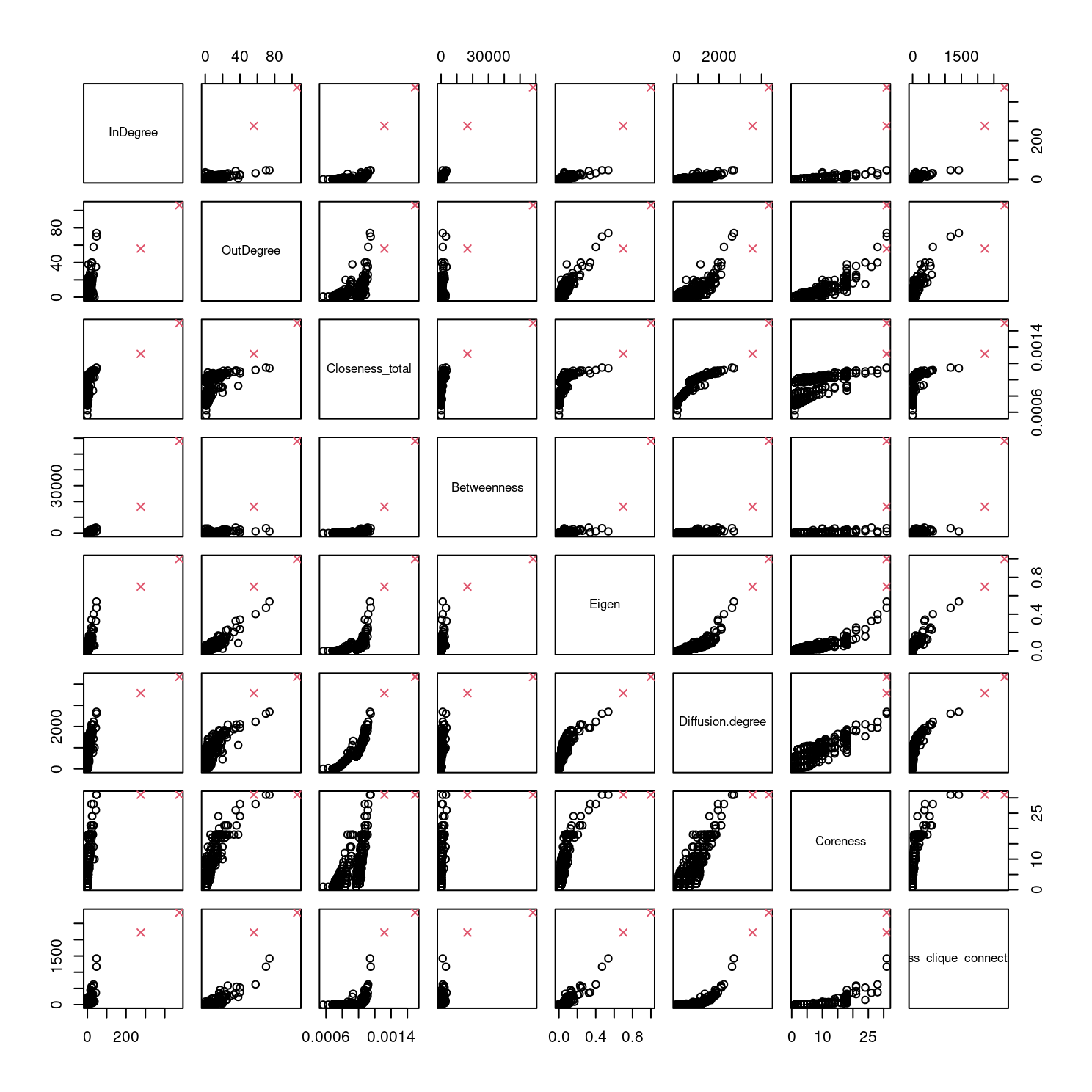
From the plots in Figure 8.1, we can see that there are clearly two quite extreme outliers. Simple exploratory analyses (not shown) confirms that these are the final two rows of the complete data set. These observations are known to correspond to the two instructors who led the discussion. They have been marked using a red cross symbol in Figure 8.1. Though we have argued that \(K\)-Medoids is a more robust clustering method than \(K\)-Means, for example, we also remove these observations in order to avoid their detrimental effects on the \(K\)-Means output. The rows must be removed from both df and demog so that they can later be merged. With these observations included, \(K\)-Means for instance would likely add one additional cluster containing just these two observations, about whom we already know their role differs substantially from the other observations, as they are quite far from the bulk of the data in terms of squared Euclidean distance. That is not to say, however, that there will not still be outliers in df after removing these two cases.
keep_ind <- 1:(nrow(df) - 2)

df <- df |> slice(keep_ind)
demog <- demog |> slice(keep_ind)
As is good practice when using dissimilarity-based clustering algorithms, we pre-process the purely continuous data by normalising each variable to have a mean of 0 and a variance of 1, by constructing the scaled data frame sdf using the function scale(), again excluding the name column.
sdf <- scale(df[,-1], center=TRUE, scale=TRUE)The object sdf can be used for all clustering methods described herein. To also accommodate the categorical demographic variables, we use merge() to combine both the scaled continuous data and the categorical data. This requires some manipulation of the name column, with which the two data sets are merged, but we ultimately discard the superfluous name column, which we do not want to contribute to any pairwise distance matrices or clustering solutions, from both merged_df and sdf.
merged_df <- data.frame(name=df$name, sdf) |>
  merge(demog, by=1) |>
  select(-name)
Finally, before proceeding to apply various clustering methods to these data, we present summaries of the counts of each level of the categorical variables experience, gender, and region. These variables imply groupings of size three, two, and five, respectively, and it will be interesting to see if this is borne out in any of the mixed-type clustering applications.
table(merged_df$experience)
  1   2   3
118 150 171 table(merged_df$gender)
female   male
299 140 table(merged_df$region)
International       Midwest     Northeast         South          West
           32            77           110           168            52
4.2 Clustering applications
We now show how each of the clustering methods described above can be implemented in R, using these data throughout and taking care to address all practical concerns previously raised. For each method —\(K\)-Means in Section 8.4.2.1, \(K\)-Medoids in Section 8.4.2.2, and agglomerative hierarchical clustering in Section 8.4.2.3— we show clustering results following the method-specific guidelines for choosing \(K\). However, we conclude by comparing results across different methods using the average silhouette width criterion to further guide the choice of \(K\) in Section 8.4.2.4. We refrain from providing an interpretation of the uncovered clusters until Section 8.4.2.5, after the optimal clustering solution is identified.
Before we proceed, we set the seed to ensure that results relying on random number generation are reproducible.
set.seed(2024)4.2.1 \(K\)-Means application
We begin by showing a naive use of the kmeans() function, supplying only the scaled data sdf and the pre-specified number of clusters \(K\) via the centers argument. For now, we assume for no particular reason that there are \(K=3\) clusters, just to demonstrate the use of the kmeans() function and its arguments. A number of aspects of the results are printed when we examine the resulting km1 object.
km1 <- kmeans(sdf, centers=3)
km1
K-means clustering with 3 clusters of sizes 48, 129, 262
Cluster means:
InDegree OutDegree Closeness_total Betweenness Eigen
1 2.2941694 1.9432559 1.0923551 1.9697769 2.00747791
2 -0.4088814 -0.4311073 -1.4086380 -0.3975783 -0.55451137
3 -0.2189864 -0.1437536 0.4934399 -0.1651209 -0.09475944
Diffusion.degree Coreness Cross_clique_connectivity
1 1.9078646 2.1923592 2.0066265
2 -1.1038258 -0.5622732 -0.3094092
3 0.1939543 -0.1248092 -0.2152835
Clustering vector:
[1] 1 2 2 3 1 1 1 1 3 1 1 3 1 1 1 2 1 3 1 2 2 1 2 1 3 1 1 2 1 1 2 3 3 1 1 1 2
[38] 3 3 2 1 3 2 1 3 3 2 3 1 1 3 3 1 1 2 3 3 1 3 1 1 1 1 1 3 3 1 1 3 3 3 3 2 3
[75] 3 3 3 3 2 2 3 3 3 2 3 2 3 1 2 3 3 1 2 3 3 3 2 1 3 1 3 3 3 3 3 2 3 2 3 3 2
[112] 3 3 3 1 1 2 2 2 3 3 2 2 3 2 3 3 3 3 2 3 2 3 3 2 3 1 3 3 2 3 3 3 3 2 3 3 3
[149] 2 3 2 3 2 3 3 2 3 3 2 3 3 3 3 2 3 3 3 2 3 3 3 3 3 2 2 3 3 3 3 2 3 2 3 3 3
[186] 3 3 3 3 3 2 3 3 3 3 3 2 1 3 3 3 3 3 3 3 3 3 2 2 2 3 3 2 3 2 2 3 3 1 2 3 2
[223] 1 2 2 3 2 2 2 2 2 3 2 1 3 3 2 2 3 3 3 3 3 2 3 3 3 3 3 3 3 3 3 2 3 3 3 3 3
[260] 2 3 2 2 2 3 2 3 2 2 2 3 2 2 2 2 3 2 3 3 3 3 2 2 3 2 2 2 2 2 2 2 3 2 2 3 2
[297] 3 3 3 3 3 3 3 3 3 2 2 3 2 1 2 2 2 3 2 2 3 3 2 3 2 3 2 3 3 3 2 2 3 3 3 2 3
[334] 2 3 3 3 3 3 3 3 3 3 3 3 3 3 2 2 3 2 2 2 3 3 3 3 3 2 3 3 3 3 3 3 3 3 3 3 2
[371] 3 3 3 3 3 3 3 3 3 3 3 3 3 3 3 3 3 3 3 3 3 3 3 3 3 3 3 3 3 3 3 3 3 3 3 3 3
[408] 3 3 3 3 3 3 3 3 2 2 2 2 2 2 2 2 3 3 3 3 3 3 3 3 1 2 2 2 2 2 2 3
Within cluster sum of squares by cluster:
[1] 858.90295 72.01655 414.30502
(between_SS / total_SS = 61.6 %)
Available components:
[1] "cluster" "centers" "totss" "withinss" "tot.withinss"
[6] "betweenss" "size" "iter" "ifault" Among other things, this output shows the estimated centroid vectors \(\boldsymbol{\mu}_1,\ldots,\boldsymbol{\mu}_K\) upon convergence of the algorithm ($centers), an indicator vector showing the assignment of each observation to one of the \(K=3\) clusters ($cluster), the size of each cluster in terms of the number of allocated observations ($size), the within-cluster sum-of-squares per cluster ($withinss), and the ratio of the between-cluster sum-of-squares ($betweenss) to the total sum of squares ($totss). Ideally, this ratio should be large, if the total within-cluster sum-of-squares is minimised. We can access the TWCSS quantity by typing
km1$tot.withinss[1] 1345.225However, these results were obtained using the default values of ten maximum iterations (iter.max=10, by default) and only one random set of initial centroid vectors (nstart=1, by default). To increase the likelihood of converging to the global minimum, it is prudent to increase iter.max and nstart, to avoid having the algorithm terminate prematurely and avoid converging to a local minimum, as discussed in Section 8.3.1.2.2. We use nstart=50, which is reasonably high but not so high as to incur too large a computational burden.
km2 <- kmeans(sdf, centers=3, nstart=50, iter.max=100)
km2$tot.withinss
[1] 1339.226We can see that the solution associated with the best random starting values achieves a lower TWCSS than the earlier naive attempt. Next, we see if an even lower value can be obtained using the \(K\)-Means initialisation strategy, by invoking the kmeans_pp() function from Section 8.3.1.2.2 with K=3 centers and supplying these centroid vectors directly to kmeans(), rather than indicating the number of random centers to use.
km3 <- kmeans(sdf, centers=kmeans_pp(sdf, K=3), iter.max=100)
km3$tot.withinss
[1] 1343.734In this case, using the \(K\)-Means initialisation strategy did not further reduce the TWCSS; in fact it is worse than the solution obtained using nstart=50. However, recall that \(K\)-Means is itself subject to randomness and should therefore also be run several times, though the number of \(K\)-Means runs need not be so high as 50. In the code below, we use replicate() to invoke both kmeans_pp() and kmeans() itself ten times in order to obtain a better solution.
KMPP <- replicate(10, list(kmeans(sdf, iter.max=100,
                                  centers=kmeans_pp(sdf, K=3))))
Among these ten solutions, five are identical and achieve the same minimum TWCSS value.
TWCSS <- sapply(KMPP, "[[", "tot.withinss")
TWCSS
[1] 1345.225 1339.226 1339.226 1339.226 1340.457 1339.226 1345.225 1345.225
[9] 1345.225 1339.226Thereafter, we can extract a solution which minimises the tot.withinss as follows:
km4 <- KMPP[[which.min(TWCSS)]]
km4$tot.withinss
[1] 1339.226Finally, this approach resulted in an identical solution to km2 being obtained — with just ten runs of \(K\)-Means and \(K\)-Means rather than nstart=50 runs of the \(K\)-Means algorithm alone— which is indeed superior to the solution obtained with just one uninformed random start in km1. We will thus henceforth adopt this initialisation strategy always.
To date, the \(K\)-Means algorithm has only been ran with the fixed number of clusters \(K=3\), which may be suboptimal. The following code iterates over a range of \(K\) values, storing both the kmeans() output itself and the TWCSS value for each \(K\). The range \(K=1,\ldots,10\) notably includes \(K=1\), corresponding to no group structure in the data. The reason for storing the kmeans() output itself is to avoid having to run kmeans() again after determining the optimal \(K\) value; such a subsequent run may not converge to the same minimised TWCSS and having to run the algorithm again would be computationally wasteful.
K <- 10 # set upper limit on range of K values

TWCSS <- numeric(K) # allocate space for TWCSS estimates

KM <- list() # allocate space for kmeans() output

for(k in 1:K) { # loop over k=1,...,K

  # Run K-means using K-Means++ initialisation:
  # use the current k value and do so ten times if k > 1
  KMPP    <- replicate(ifelse(k > 1, 10, 1),
                       list(kmeans(sdf, iter.max=100,
                                   centers=kmeans_pp(sdf, K=k))))

  # Extract and store the solution which minimises the TWCSS
  KM[[k]] <- KMPP[[which.min(sapply(KMPP, "[[", "tot.withinss"))]]

  # Extract the TWCSS value for the current value of k
  TWCSS[k] <- KM[[k]]$tot.withinss
}
As previously stated in Section 8.3.1.2.1, the so-called “elbow method” consists of plotting the range of \(K\) values on the x-axis against the corresponding obtained TWCSS values on the y-axis and looking for an kink in the resulting curve.
plot(x=1:K, y=TWCSS, type="b",
     xlab="K", ylab="Total Within-Cluster\n Sum-of-Squares")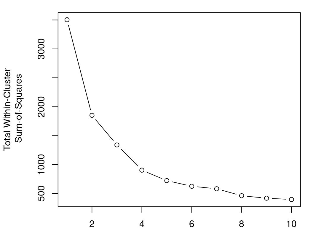
Here, it appears that \(K=4\) would produce the best results: beyond \(K=4\), the decrease in TWCSS is minimal, which suggests that an extra cluster is not required to model the data well; between \(K=3\) and \(K=4\), there is a more substantial decrease in TWCSS, which suggests that the fourth cluster is necessary. This method is of course highly subjective, and we will further inform our choice of \(K\) for \(K\)-Means using silhouette widths and the ASW criterion in Section 8.4.2.4.
For now, we can interrogate the \(K\)-Means solution with \(K=4\) by examining the sizes of the clusters and their centroid vectors, using the corresponding fourth element of the list KM by setting K <- 4.
K <- 4

KM[[K]]$size
[1] 127 57 8 247KM[[K]]$centers InDegree OutDegree Closeness_total Betweenness Eigen Diffusion.degree
1 -0.4086612 -0.4381057 -1.4220978 -0.3994123 -0.5596480 -1.1138889
2 1.5706416 1.1372352 0.9247804 1.3859592 1.0781087 1.4216179
3 4.1035975 5.0512503 1.5201941 3.4673658 5.4946785 3.1631065
4 -0.2852445 -0.2007813 0.4685522 -0.2267743 -0.1390054 0.1422138
Coreness Cross_clique_connectivity
1 -0.5672245 -0.3102236
2 1.7423739 0.9615041
3 3.4821417 5.5033583
4 -0.2232184 -0.2406243However, these centroids correspond to the scaled version of the data created in Section 12.4.3. Interpretation can be made more straightforward by undoing the scaling transformation on these centroids, so that they are on the same scale as the data df rather than the scaled data sdf which was used as input to kmeans(). The column-wise means and standard deviations used when scale() was invoked are available as the attributes "scaled:center" and "scaled:scale", respectively and are used in the code below. We show these centroids rounded to four decimal places in Table 8.1.
rescaled_centroids <- t(apply(KM[[K]]$centers, 1, function(r) {
                        r * attr(sdf, "scaled:scale") + attr(sdf, "scaled:center")
                        } ))
round(rescaled_centroids, 4)| InDegree | OutDegree | Closeness_total | Betweenness | Eigen | Diffusion.degree | Coreness | Cross_clique_connectivity |
|---|---|---|---|---|---|---|---|
| 1.1024 | 1.7480 | 0.0008 | 20.7010 | 0.0071 | 144.1732 | 2.6378 | 4.6850 |
| 15.3684 | 14.8421 | 0.0010 | 849.9328 | 0.0996 | 1370.1053 | 16.1053 | 157.5789 |
| 33.6250 | 47.3750 | 0.0011 | 1816.6608 | 0.3492 | 2212.1250 | 26.2500 | 703.6250 |
| 1.9919 | 3.7206 | 0.0010 | 100.8842 | 0.0308 | 751.5061 | 4.6437 | 13.0526 |
Now, we can more clearly see that the first cluster, with \(n_{k=1}=127\) observations, has the lowest mean value for all \(d=8\) centrality measures, while the last cluster, the largest with \(n_{k=4}=247\) observations, has moderately larger values for all centrality measures. The two smaller clusters, cluster two with \(n_{k=2}=57\) observations and cluster three with only \(n_{k=3}=8\) observations have the second-largest and largest values for each measure, respectively. As previously stated, we defer a more-detailed interpretation of uncovered clusters to Section 8.4.2.5, after the optimal clustering solution has been identified.
4.2.2 \(K\)-Medoids application
The function pam() in the cluster library implements the PAM algorithm for \(K\)-Medoids clustering. By default, this function requires only the arguments x (a pre-computed pairwise dissimilarity matrix, as can be created from the functions dist(), daisy(), and more) and k, the number of clusters. However, there are many options for many additional speed improvements and initialisation strategies [48]. Here, we invoke a faster variant of the PAM algorithm which necessitates specification of nstart as a number greater than one, to ensure the algorithm is evaluated with multiple random initial medoid vectors, in a similar fashion to kmeans(). Thus, we call pam() with variant="faster" and nstart=50 throughout.
Firstly though, we need to construct the pairwise dissimilarity matrices to be used as input to the pam() function. Unlike \(K\)-Means, we are not limited to squared Euclidean distances. It is prudent, therefore, to explore \(K\)-Medoids solutions with several different dissimilarity measures and compare the different solutions obtained for different measures. Each distance measure will yield different results at the same \(K\) value, thus the value of \(K\) and the distance measure must be considered as a pair when determining the optimal solution.
We begin by calculating the Euclidean, Manhattan, and Minkowski (with \(p=3\)) distances on the scaled continuous data in sdf:
dist_euclidean <- dist(sdf, method="euclidean")

dist_manhattan <- dist(sdf, method="manhattan")

dist_minkowski3 <- dist(sdf, method="minkowski", p=3)
Secondly, we avail of another principal advantage of \(K\)-Medoids; namely, the ability to incorporate categorical variables in mixed-type data sets, by calculating pairwise Gower distances between each row of merged_df, using daisy().
dist_gower <- daisy(merged_df, metric="gower")As per the \(K\)-Means tutorial in Section 8.4.2.1, we can produce an elbow plot by running the algorithm over a range of \(K\) values and extracting the minimised within-cluster total distance achieved upon convergence for each value of \(K\). We demonstrate this for the dist_euclidean input below.
K <- 10
WCTD_euclidean <- numeric(K)
pam_euclidean <- list()
for(k in 1:K) {
pam_euclidean[[k]] <- pam(dist_euclidean, k=k, variant="faster", nstart=50)
WCTD_euclidean[k] <- pam_euclidean[[k]]$objective[2]
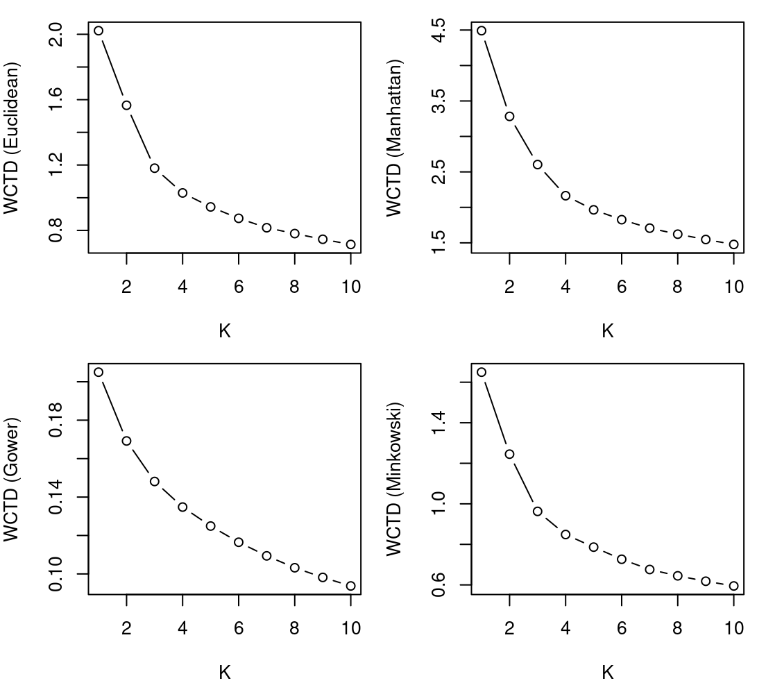
}Equivalent code chunks for the dist_manhattan, dist_minkowski3, and dist_gower inputs are almost identical, so we omit them here for the sake of brevity. Suffice to say, equivalent lists pam_manhattan, pam_minkowski3, and pam_gower, as well as equivalent vectors WCTD_manhattan, WCTD_minkowski3, and WCTD_gower, can all be obtained. Using these objects, corresponding elbow plots for all four dissimilarity measures are showcased in Figure 8.3.
Some of the elbow plots in Figure 8.3 are more conclusive than others. As examples, there are reasonably clear elbows at \(K=3\) for the Euclidean and Minkowski distances, arguably an elbow at \(K=4\) for the Manhattan distance, and no clear, unambiguous elbow under the Gower distance. In any case, the elbow method only helps to identify the optimal \(K\) value for a given dissimilarity measure; we defer a discussion of how to choose the overall best \(K\)-Medoids clustering solution to later in this tutorial.
For now, let’s interrogate the \(K=3\) solution obtained using the Euclidean distance. Recall that the results are already stored in the list pam_euclidean, so we merely need to access the third component of that list by setting K <- 3. Firstly, we can examine the size of each cluster by tabulating the cluster-membership indicator vector as follows:
K <- 3

table(pam_euclidean[[K]]$clustering)
  1   2   3
 67 122 250
Examining the medoids which serve as prototypes of each cluster is rendered difficult by virtue of the input having been a distance matrix rather than the data set itself. Though \(K\)-Medoids defines the medoids to be the rows in the data set from which the distance to all other observations currently allocated to the same cluster, according to the specified distance measure, is minimised, the medoids component of the output instead gives the indices of the medoids within the data set.
pam_euclidean[[K]]$medoids[1] 88 272 45Fortunately, these indices within sdf correspond to the same, unscaled observations within df. Allowing for the fact that observations with name greater than the largest index here were removed due to missingness, they are effectively the values of the name column corresponding to the medoids. Thus, we can easily examine the medoids on their original scale. In Table 8.2, they include the name column, which was not used when calculating the pairwise distance matrices, and are rounded to four decimal places.
df |>
  slice(as.numeric(pam_euclidean[[K]]$medoids)) |>
round(4)| name | InDegree | OutDegree | Closeness_total | Betweenness | Eigen | Diffusion.degree | Coreness | Cross_clique_connectivity |
|---|---|---|---|---|---|---|---|---|
| 88 | 16 | 14 | 0.0011 | 675.5726 | 0.1096 | 1415 | 18 | 157 |
| 272 | 1 | 1 | 0.0007 | 0.0000 | 0.0047 | 41 | 2 | 2 |
| 45 | 1 | 2 | 0.0010 | 29.4645 | 0.0194 | 684 | 3 | 5 |
Thus, we can see that there is a small cluster with \(n_{k=1}=67\) observations which has the largest values for all \(d=8\) centrality measures, a slightly larger cluster with \(n_{k=2}=122\) observations and the lowest values for all variables, and the largest cluster with \(n_{k=3}=250\) and intermediate values for all variables. The cluster sizes of the \(K\)-Medoids solution being more evenly balanced than the earlier \(K\)-Means solution is an artefact of \(K\)-Medoids being less susceptible to outlying observations by virtue of not squaring the distances. We can explore this by cross-tabulating the clusters obtained by \(K\)-Means with \(K=4\) and \(K\)-Medoids with \(K=3\) and the Euclidean distance in Table 8.3.
table(pam_euclidean[[3]]$clustering,
KM[[4]]$cluster)| 1 | 2 | 3 | 4 | ||
| 1 | 0 | 57 | 8 | 2 | |
| 2 | 122 | 0 | 0 | 0 | |
| 3 | 5 | 0 | 0 | 245 |
From the cross-tabulation in Table 8.3, we can see that the \(n_k=8\) observations in the smallest \(K\)-Means cluster were absorbed into a larger cluster under the \(K\)-Medoids solution, thereby demonstrating the robustness of \(K\)-Medoids to outliers. Otherwise, both solutions are broadly in agreement.
4.2.3 Agglomerative hierarchical clustering application
Performing agglomerative hierarchical clustering is straightforward now that the distance matrices have already been created for the purposes of running pam(). All that is required is to specify the distance matrix and an appropriate linkage criterion as the method when calling hclust(). We demonstrate this below for a subset of all possible distance measure and linkage criterion combinations among those described in Section 8.3.2.1. Recall that for the Ward criterion, the underlying distance measure is usually assumed to be squared Euclidean and that "ward.D2" is the correct method to use when the Euclidean distances are not already squared. For method="centroid", we manually square the Euclidean distances.
hc_minkowski3_complete <- hclust(dist_minkowski3, method="complete")

hc_manhattan_single <- hclust(dist_manhattan, method="single")

hc_gower_average <- hclust(dist_gower, method="average")

hc_euclidean_ward <- hclust(dist_euclidean, method="ward.D2")

hc_euclidean2_centroid <- hclust(dist_euclidean^2, method="ward.D2")
Plotting the resulting dendrograms is also straightforward. Simply calling plot() on any of the items above will produce a dendrogram visualisation. We do so here for four of the hierarchical clustering solutions constructed above —the undepicted hc_euclidean2_centroid dendrogram is virtually indistinguishable from that of hc_euclidean_ward— while suppressing the observation indices along the x-axis for clarity by specifying labels=FALSE.
plot(hc_minkowski3_complete, labels=FALSE,
     main="", xlab="Minkwoski Distance (p=3) with Complete Linkage")
plot(hc_manhattan_single, labels=FALSE,
     main="", xlab="Manhattan Distance with Single Linkage")
plot(hc_gower_average, labels=FALSE,
     main="", xlab="Gower Distance with Average Linkage")
plot(hc_euclidean_ward, labels=FALSE,
     main="", xlab="Euclidean Distance with the Ward Criterion")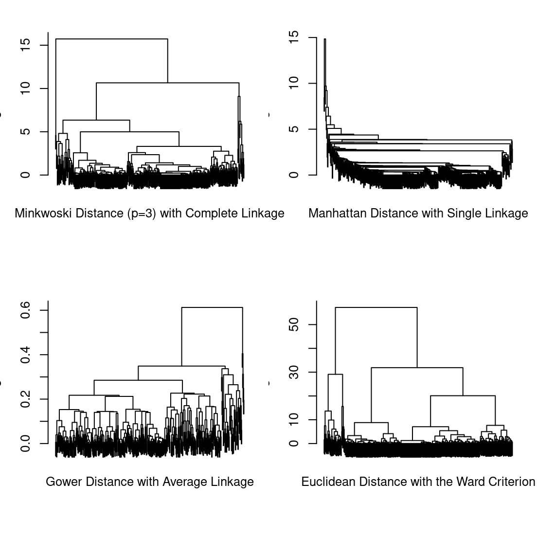
As previously alluded to in Section 8.3.2.2, some combinations of dissimilarity measure and linkage criterion are liable to produce undesirable results. The susceptibility to outliers of complete linkage clustering is visible in the top-left panel of Figure 8.4, where just two observations form a cluster at a low height and are never again merged. The tendency of single linkage clustering to exhibit a “chaining” effect whereby all observations are successively merged into just one ever-larger cluster is evident in the top-right panel of Figure 8.4, and similar behaviour is observed for the Gower distance with average linkage depicted in the bottom-left panel. The most reasonable results appear to arise from using the Ward criterion in conjunction with Euclidean distances.
Taking the set of candidate partitions in hc_euclidean_ward, for the reasons outlined above, all that remains is to cut this dendrogram at an appropriate height. Practitioners have the freedom to explore different levels of granularity in the final partition. Figure 8.5 shows the dendrogram from the bottom-right panel of Figure 8.4 cut horizontally at different heights, indicated by lines of different colours, as well as the corresponding implied \(K\) values.
Thereafter, one simply extracts the resulting partition by invoking cutree() with the appropriate height h. For example, to extract the clustering with \(K=3\), which we choose here because of the wide range of heights at which a \(K=3\) solution could be obtained:
hc_ward2 <- cutree(hc_euclidean_ward, h=45)The object hc_ward2 is now simply an vector indicating the cluster-membership of each observation in the data set. We show only the first few, for brevity, and then tabulate this vector to compute the cluster sizes. However, interpretation of these clusters is more difficult than in the case of \(K\)-Means and \(K\)-Medoids, as there is no centroid or medoid prototype with which to characterise each cluster.
head(hc_ward2)[1] 1 2 2 2 1 1table(hc_ward2)hc_ward2
1 2
49 390 In this section, we have not presented an exhaustive evaluation of all possible pairs of dissimilarity measure and linkage criterion, but note that the code to do so is trivial. In any case, much like \(K\)-Means and \(K\)-Medoids, we must turn to other cluster quality indices to guide the choice of the best overall solution, be that choosing the best distance and linkage settings for agglomerative hierarchical clustering, or choosing the best clustering method in general among several competing methods. We now turn to finding the optimal clustering solution among multiple competing methods, guided by silhouette widths and plots thereof.
4.2.4 Identifying the optimal clustering solution
In our application of \(K\)-Means, the elbow method appeared to suggest that \(K=4\) yielded the best solution. In our applications of \(K\)-Medoids, the elbow method suggested different values of \(K\) for different distance metrics. Finally, in our applications of hierarchical clustering, we noted that visualising the resulting dendrogram could be used to guide the choice of the height at which to cut to produce a single hard partition of \(K\) clusters. Now, we must determine which method yields the overall best solution. Following Section 8.3.3, we employ silhouettes for this purpose.
For \(K\)-Means and agglomerative hierarchical clustering, silhouettes can be computed using the silhouette function in the cluster library, in which case the function requires two arguments; the integer vector containing the cluster membership labels and an appropriate dissimilarity matrix. Thus, for instance, silhouettes could be obtained easily for the following two examples (using kmeans() and hclust(), respectively).
kmeans_sil <- silhouette(kmeans(sdf, centers=kmeans_pp(sdf, K=4),
                                iter.max=100)$cluster,
                         dist_euclidean)
hclust_sil <- silhouette(cutree(hclust(dist_euclidean, method="ward.D2"), k=2),
dist_euclidean)For \(K\)-Medoids, it suffices only to supply the output of pam() itself, from which the cluster membership labels and appropriate dissimilarity matrix will be extracted internally, e.g.,
pam_sil <- silhouette(pam(dist_euclidean, k=3, variant="faster", nstart=50))Thereafter, plot() can be called on kmeans_sil, hclust_sil, or pam_sil to produce a silhouette plot. For an example based on hclust_sil, see Figure 8.6. Note that as \(K=2\) here, col=2:3 colours the silhouettes according to their cluster.
plot(hclust_sil, main="", col=2:3)
Figure 8.6 shows that most silhouette widths are positive under this solution, indicating that most observations have been reasonably well-clustered. Cluster 2 appears to be the most cohesive, with a cluster-specific average silhouette width of \(0.70\), while cluster 1 appears to be the least cohesive, with a corresponding average of just \(0.24\). The overall ASW is \(0.65\), as indicated at the foot of the plot.
Given that we adopted a range of \(K=1,\ldots,10\) when using \(K\)-Means and \(K\)-Medoids, and four different dissimilarity measures when using \(K\)-Medoids, we have \(50\) non-hierarchical candidate solutions to evaluate, of which some seem more plausible than others according to the respective elbow plots. For agglomerative hierarchical clustering, an exhaustive comparison over a range of \(K\) values, for each dissimilarity measure and each linkage criterion, would be far too extensive for the present tutorial. Consequently, we limit our evaluation of silhouettes to the \(K\)-Means and \(K\)-Medoids solutions already present in the objects KM, pam_euclidean, pam_manhattan, pam_minkowski3, and pam_gower, and the hierarchical clustering solutions which employ the Ward criterion in conjunction with Euclidean distances (of which we consider a further \(10\) solutions, again with \(K=1,\ldots,10\), by considering the \(10\) possible associated heights at which the dendrogram can be cut). We limit the hierarchical clustering solutions to those based on the Ward criterion given that single linkage and complete linkage have been shown to be susceptible to chaining and sensitive to outliers, respectively. We use the corresponding pre-computed dissimilarity matrices dist_euclidean, dist_manhattan, dist_minkowski3, and dist_gower, where appropriate throughout.
Though the ASW associated with hclust_sil is given on the associated silhouette plot in Figure 8.6, we can calculate ASW values for other solutions —which we must do to determine the best solution— without producing individiual silhouette plots. To show how this can be done, we examine the structure of the hclust_sil object, showing only its first few rows.
head(hclust_sil) cluster neighbor sil_width
[1,] 1 2 0.4408007
[2,] 2 1 0.7416708
[3,] 2 1 0.7401549
[4,] 2 1 0.4696606
[5,] 1 2 0.2494557
[6,] 1 2 0.1915306The columns relate to the cluster to which object \(i\) is assigned, the cluster for which the corresponding \(b(i)\) was minimised, and the \(s(i)\) score itself, respectively. Calculating mean(hclust_sil[,3]) will return the ASW. Though the code is somewhat tedious, we calculate the ASW criterion values for all \(60\) candidate solutions —that is, six methods evaluated over \(K=1,\ldots,10\)— using a small helper function to calculate the ASW for the sake of tidying the code.
K <- 10
ASW <- function(x) mean(x[,3])
silhouettes <- data.frame(K=2:K,
  kmeans=sapply(2:K, function(k) ASW(silhouette(KM[[k]]$cluster, dist_euclidean))),
  kmedoids_euclidean=sapply(2:K, function(k) ASW(silhouette(pam_euclidean[[k]]))),
  kmedoids_manhattan=sapply(2:K, function(k) ASW(silhouette(pam_manhattan[[k]]))),
  kmedoids_minkowski3=sapply(2:K, function(k) ASW(silhouette(pam_minkowski3[[k]]))),
  kmedoids_gower=sapply(2:K, function(k) ASW(silhouette(pam_gower[[k]]))),
  hc_euclidean_ward=sapply(2:K, function(k) ASW(silhouette(cutree(hc_euclidean_ward,
                                                             k), dist_euclidean))))
In Figure 8.7, we plot these silhouettes against \(K\) using matplot(), omitting the code to do so for brevity.
According to Figure 8.7, there is generally little support for \(K > 5\) across almost all methods considered, as most method’s ASW values begin to decline after this point. The ASW values also make clear that incorporating the additional categorical demographic variables in a mixed-type clustering using the Gower distance does not lead to reasonable partitions, for any number of clusters \(K\). Overall, the most promising solutions in terms of having the highest ASW are \(K\)-Means, Ward hierarchical clustering, and \(K\)-Medoids with the Manhattan distance, all with \(K=2\), and \(K\)-Medoids with the Euclidean and Minkowski distances, each with \(K=3\). However, it would be wise to examine silhouette widths in more detail, rather than relying merely on the average. The silhouettes for this hierarchical clustering solution are already depicted in Figure 8.6, so Figure 8.8 shows individual silhouette widths for the remaining solutions.
It is notable that the silhouettes and ASW of the \(K=2\) \(K\)-Means solution (top-left panel of Figure 8.8) and the Ward hierarchical clustering solution (Figure 8.6) appear almost identical (if one accounts for the clusters being relabelled and associated colours being swapped). Indeed, according to a cross-tabulation of their partitions (not shown), their assignments differ for just \(4\) out of \(n=439\) observations. Despite having the highest ASW, we can justify dismissing these solutions given that \(K=2\) was not well-supported by its corresponding elbow plot in Figure 8.2. Similar logic suggests that the \(K=3\) \(K\)-Means solution and the \(K=2\) \(K\)-Medoids solution based on the Manhattan distance can also be disregarded. Although we stress again that an ideal analysis would more thoroughly determine an optimal solution with reference to additional cluster quality measures and note that various clustering solutions can be legitimate, for potentially different clustering aims, on the same data set [2, 3], we can judge that —among the two \(K=3\) \(K\)-Medoids solutions— the one based on the Euclidean distance is arguably preferable, for two reasons. Firstly, its ASW is quite close to that of the Minkowski distance solution:
silhouettes |>
  filter(K == 3) |>
  select(kmedoids_euclidean, kmedoids_minkowski3)
Secondly, the first cluster has a higher cluster-specific average silhouette width under the solution based on the Euclidean distance. Indeed, this solution has fewer negative silhouette widths also:
sum(silhouette(pam_euclidean[[3]])[,3] < 0)[1] 27sum(silhouette(pam_minkowski3[[3]])[,3] < 0)[1] 284.2.5 Interpreting the optimal clustering solution
By now, we have identified that the \(K=3\) solution obtained using \(K\)-Medoids and the Euclidean distance is optimal. Although aspects of this solution were already discussed in Section 8.4.2.2 —in particular, Table 8.2 has already shown the \(K=3\) medoid vectors obtained at convergence— we now turn to examining this output in greater detail, in order to provide a fuller interpretation of each of the uncovered clusters. We extract this solution for ease of manipulation.
final_pam <- pam_euclidean[[3]]Recall that this method yielded three clusters of sizes \(n_1=67\), \(n_2=122\), and \(n_3=250\). Although the categorical variables were not used by this clustering method, additional interpretative insight can be obtained by augmenting the respective medoids in Table 8.2 with these cluster sizes and the experience values of the corresponding rows of the merged_df data set, which includes the additional demographic features.
df |>
  slice(as.numeric(final_pam$medoids)) |>
  round(4) |>
  mutate(size=table(final_pam$clustering)) |>
  left_join(slice(demog |>
                    select(UID, experience),
                  as.numeric(final_pam$medoids)),
            by=join_by(name == UID)) |>
select(-name)| InDegree | OutDegree | Closeness_total | Betweenness | Eigen | Diffusion.degree | Coreness | Cross_clique_connectivity | size | experience |
|---|---|---|---|---|---|---|---|---|---|
| 16 | 14 | 0.0011 | 675.5726 | 0.1096 | 1415 | 18 | 157 | 67 | 1 |
| 1 | 1 | 0.0007 | 0.0000 | 0.0047 | 41 | 2 | 2 | 122 | 3 |
| 1 | 2 | 0.0010 | 29.4645 | 0.0194 | 684 | 3 | 5 | 250 | 2 |
Interpretation and labeling of the clustering results is the step that follows, with a focus only on the medoid values of the centrality scores (had the optimal solution been obtained by kmeans(), we could instead examine its centroids in its $centers component, i.e., mean vectors). We will follow the example papers that we used as a guide for choosing the centrality measures [28] and [61]. Both papers have used traditional centrality measures (e.g., degree, closeness, and betweenness) as well as diffusion centralities (diffusion degree and coreness) to infer students’ roles. Furthermore, the second paper has an extended review of the roles and how they have been inferred from centrality measures, so readers are encouraged to read this review.
As the data shows, the first cluster has the highest degree centrality measures (InDegree and OutDegree), highest betweenness centrality, as well as the highest values of the diffusion centralities (Diffusion_degree and Coreness). These values are concordant with students who were actively engaged, received multiple replies, had their contributions discussed by others, and achieved significant diffusion. All of such criteria are concordant with the role of leaders. It stands to reason that the leaders cluster would be the smallest, with \(n_1=67\).
The third cluster has intermediate values for the degree centralities, high diffusion centrality values, as well as relatively high values of betweenness centrality. Such values are concordant with the role of an active participant who participates and coordinates the discussion. Therefore, we will use the label of coordinators.
Finally, the second cluster has the lowest values for all centrality measures (though its diffusion values are still fairly reasonable). Thus, this cluster could feasibly be labelled as an isolates cluster, gathering participants whose role in the discussions is peripheral at best. Overall, the interpretations of this \(K=3\) solution are consistent with other findings in the existing literature, e.g., [28].
We can now label the clusters accordingly to facilitate more informative cluster-specific summaries. Here, we also recall the size of each cluster with the new labels invoked, to demonstrate their usefulness.
final_pam$clustering <- factor(final_pam$clustering,
                               labels=c("leaders", "coordinators", "isolates"))
table(final_pam$clustering)
     leaders coordinators     isolates
          67          122          250
As an example, we can use these labels to guide a study of the mean vectors of each cluster(bearing in mind that these are not centroid centroid vectors obtained by \(K\)-Means, but rather mean vectors obtained calculated for each group defined by the \(K\)-Medoids solution), for which the interpretation of the leader, coordinator, and isolate labels are still consistent with the conclusions drawn from the medoids in Table 8.2. Note that, for the sake of readability, the group-wise summary below is transposed.
df |>
  group_by(clusters=final_pam$clustering) |>
  select(-name) |>
  summarise_all(mean) |>
  mutate_if(is.numeric, round, 2) |>
  pivot_longer(cols=-clusters,
               names_to="centrality") |>
  pivot_wider(names_from=clusters,
              values_from=value)
From Table 8.4, we can also see that each observation which corresponds to a cluster medoid contains low, high, and medium levels of experience, respectively. However, one should be cautious not to therefore conclude that the clusters neatly map to experience levels, as the following cross-tabulation indicates little-to-no agreement between the groupings of experience levels in the data and the uncovered clusters.
table(final_pam$clustering,
      merged_df$experience,
      dnn=c("Clusters", "Experience"))
Experience
Clusters 1 2 3
leaders 17 23 27
coordinators 40 34 48
isolates 61 93 96Finally, we can produce a visualisation of the uncovered clusters in order to better understand the solution. Visualising multivariate data with \(d>2\) is challenging and consequently such visualisations must resort to either plotting the first two principal components or mapping the pairwise dissimilarity matrix to a configuration of points in Cartesian space using multidimensional scaling. The latter is referred to as a “CLUSPLOT” [62] and is implemented in the clusplot() function in the same cluster library as pam() itself. This function uses classical (metric) multi-dimensional scaling [63] to create a bivariate plot displaying the partition of the data. Observations are represented by points in the scatter plot an ellipse spanning the smallest area containing all points in the given cluster is drawn around each cluster. In the code below, only clusplot(final_pam) is strictly necessary to produce such a plot for the optimal \(K=3\) Euclidean distance \(K\)-Medoids solution; all other arguments are purely for cosmetic purposes for the sake of the resulting Figure 8.9 and are described in ?clusplot.
Figure 8.9 shows that the leaders cluster —the smallest cluster with the highest value for all centrality measures— is quite diffuse. Conversely, the larger coordinators cluster, with the smallest values for all centrality measures, and the isolates cluster, the largest of all, with intermediate values for all centrality measures, are more compact. This is consistent with the cluster-specific average silhouette widths shown in the bottom-right panel of Figure 8.8. That being said, the large span of the leaders cluster again affirms the relative robustness of \(K\)-Medoids to outliers, of which some (all of which are leaders) still remain despite the earlier pre-processing steps.
clusplot(final_pam,                                    # the pam() output
         main="", sub=NA,            # remove the main title and subtitle
         lines=0,                     # do not draw any lines on the plot
         labels=4,                              # only label the ellipses
         col.clus="black",               # colour for ellipses and labels
         col.p=as.numeric(final_pam$clustering) + 1, # colours for points
         cex.txt=0.75,                      # control size of text labels
         xlim=c(-4, 17)          # expand x-axis to avoid trimming labels
         )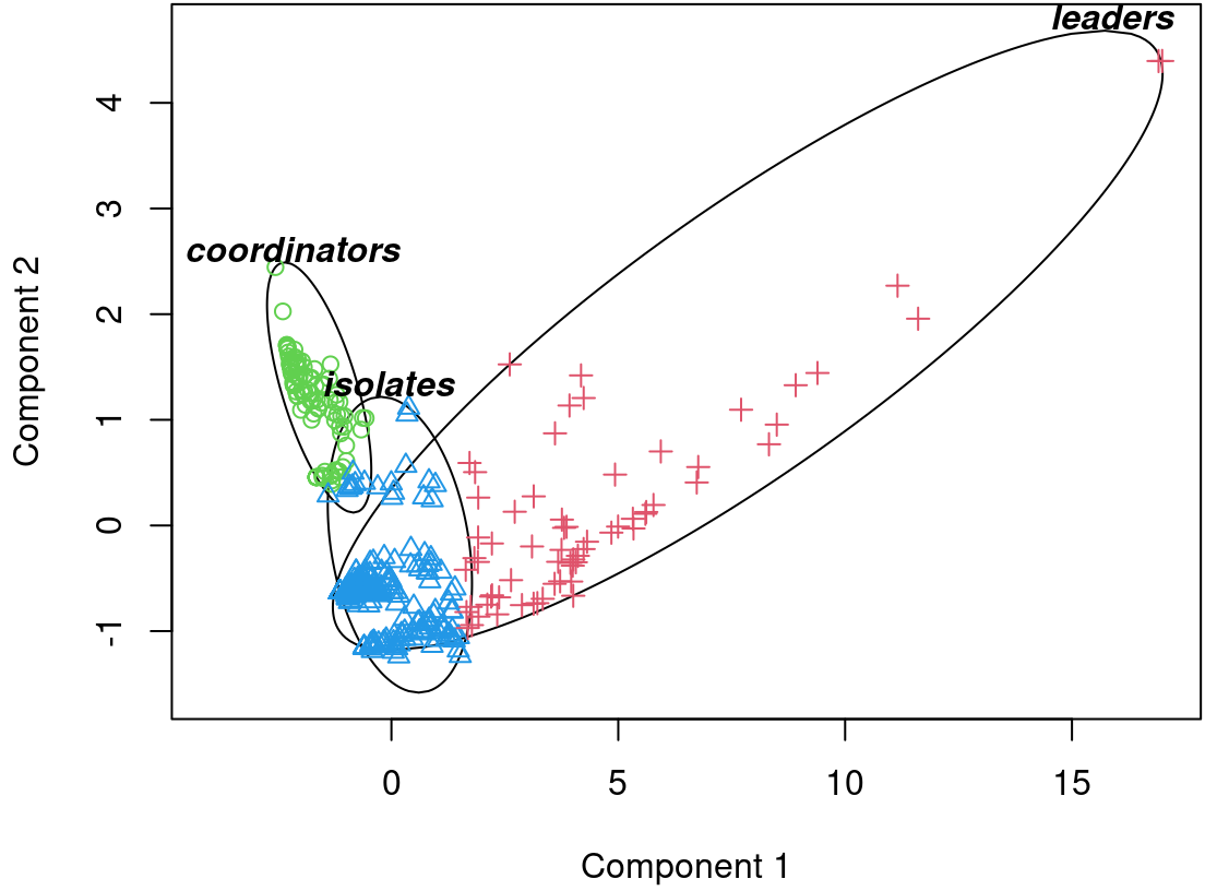
5 Discussion & further readings
The present analysis of the MOOC centralities data set incorporated three of the most commonly used dissimilarity-based clustering approaches; namely, \(K\)-Means, \(K\)-Medoids, and agglomerative hierarchical clustering. Throughout the applications, emphasis was placed on the sensitivity of the results to various choices regarding algorithmic inputs available to practitioners, be that the choice of how to choose initial centroids for \(K\)-Means, the choice of dissimilarity measure for \(K\)-Medoids, or the choice of linkage criterion for hierarchical clustering, as examples. Consequently, our analysis considered different values of \(K\), different distances, different linkage criteria, different combinations thereof, and indeed different clustering algorithms entirely, in an attempt to uncover the “best” clustering solution for the MOOC centralities data set. We showed how elbow plots and other graphical tools can guide the choice of \(K\) for a given method but ultimately identified —via the average silhouette width criterion— an optimal solution with \(K=3\), using \(K\)-Medoids in conjunction with the Euclidean distance measure. Although we note that there are a vast array of other cluster quality measures in the literature which target different definitions of what constitutes a “good” clustering [3], the solution we obtained seems reasonable, in that the uncovered clusters which we labelled as leaders, coordinators, and isolates are consistent, from an interpretative point of view, with existing educational research. Indeed, several published studies have uncovered similar patterns of three groups which can be labelled in the same way [28, 64, 65].
Nonetheless, there are some limitations to our applications of dissimilarity-based clustering methods in this tutorial which are worth mentioning. Firstly, we note firstly that the decision to standardise the variables —in particular, to normalise them by subtracting their means and dividing by their standard deviations— was applied across the board to each clustering method we explored. Although the standardised data were only used as inputs to each algorithm (i.e., the output was always interpreted on the original scale), we note that different groups are liable to be uncovered with different standardisation schemes. In other words, not standardising the data, or using some other standardisation method (e.g., rescaling to the \([0,1]\) range) may lead to different, possibly more or less meaningful clusters.
A second limitation is that all variables in the data were used as inputs (either directly in the case of \(K\)-Means, or indirectly as inputs to the pairwise dissimilarity matrix calculations required for \(K\)-Medoids and hierarchical clustering). As well as increasing the computational burden, using all variables can be potentially problematic in cases where the clustering structure is driven by some \(d^\star< d\) variables, i.e., if the data can be separated into homogeneous subgroups along fewer dimensions. In such instances where some of the variables are uninformative in terms of explaining the variability in the data, variable selection strategies tailored to the unsupervised paradigm may be of interest and again may lead to more meaningful clusters being found [66, 67].
Although dissimilarity-based clustering encompasses a broad range of flexible methodologies which can be utilised in other, diverse settings —for example, dissimilarity-based clustering is applied in the context of longitudinal categorical data in the chapter on sequence analysis methods [Chapter 10; [18]]— there are other clustering paradigms which may be of interest in similar or alternative settings as the data used in the present tutorial, even if they are not yet widely adopted in educational research. We now briefly introduce some of these alternative clustering frameworks for readers interested in expanding their knowledge of the topic of clustering beyond the dissimilarity-based framework detailed herein.
A first alternative to dissimilarity-based clustering is the density-based clustering framework, most famously exemplified by the DBSCAN clustering algorithm [68, 69]. Density-based clustering broadly defines clusters as areas of higher density than the remainder of the data set, where objects are closely packed together with many nearby neighbours, while objects in the sparse areas which separate clusters are designated as outliers. This has been identified as one main advantage of DBSCAN by authors who applied it an education research context [70] —insofar as the capability to easily and effectively separate individual exceptionally poor or exceptionally outstanding students who require special attention from teachers is desirable— along with DBSCAN obviating the need to pre-specify the number of clusters \(K\).
Another alternative is given by the model-based clustering paradigm, which is further discussed in Chapter 9 [8]. Although we direct readers to that chapter for a full discussion of model-based clustering using finite Gaussian mixture models, the relationship between this approach and latent profile analysis, and a tutorial in R using the mclust package [71], there are some aspects and advantages which are pertinent to discuss here. Firstly, as model-based clustering is based on an underlying generative probability model, rather than relying on dissimilarity-based heuristics, it admits the use of principled, likelihood-based model-selection criteria such as the Bayesian information criterion [72], thereby eliminating the subjectivity of elbow plots and other graphical tools for guiding the choice of \(K\). Secondly, such models can be extended to allow covariates to guide the construction of the clusters [73], thereby enabling, for example, incorporation of the categorical demographic variables associated with the MOOC centralities data set used in the present tutorial.
A third advantage of model-based clustering is that it returns a “soft” partition, whereas dissimilarity-based approaches yield either a single “hard” partition (with each observation placed in one group only), under partitional methods like \(K\)-Means or \(K\)-Medoids, or a set of nested hard partitions from which a single hard partition can be extracted, under hierarchical clustering. Specifically, model-based clustering assigns each observation a probability of belonging to each cluster, such that observations can have a non-negative association with more than one cluster and the uncertainty of the cluster memberships can be quantified. This has the effect of diminishing the effect of outliers or observations which lie on the boundary of two or more natural clusters, as they are not forced to wholly belong to one cluster. In light of these concerns, another clustering paradigm of potential interest is that of fuzzy clustering, which is notable for allowing for “soft” cluster-membership assignments while still being dissimilarity-based [74, 75]. Indeed, there are fuzzy variants of the \(K\)-Means and \(K\)-Medoids algorithms which relax the assumption that the latent variable \(\mathbf{z}_i\) encountered in Equation 8.1, for example, is binary. They are implemented in the functions FKM() and FKM.med(), respectively, in the fclust R package [76].
Another advantage of model-based clustering over the dissimilarity-based paradigm is the flexibility it affords in relation to the shapes, orientations, volumes, and sizes of the clusters it uncovers. At their most flexible, finite Gaussian mixture models can find clusters where all of these characteristics differ between each cluster, but intermediary configurations —whereby, as but one example, clusters can be constrained to have equal volume and orientation but varying shape and size— are permissible. This is achieved via different parsimonious parameterisations of the cluster-specific covariance matrices which control the geometric characteristics of the corresponding ellipsoids; see Chapter 9 [8] for details. By contrast, \(K\)-Means is much more restrictive. The algorithm assumes that clusters are of similar size, even if the estimated clusters can vary in size upon convergence. Moreover, by relying on squared Euclidean distances to a mean vector, with no recourse to modelling covariances, \(K\)-Means implicitly assumes that all clusters are spherical in shape, have equal volume, and radiate around their centroid. This can have the damaging consequence, in more challenging applications, that a a larger number of spherical clusters may be required to fit the data well, rather than a more parsimonious and easily interpretable mixture model with fewer non-spherical components. Finally, in light of these concerns, we highlight the spectral clustering approach [77], implemented via the function specc() in the kernlab package in R, which is, like model-based clustering, capable of uncovering clusters with more flexible shapes, particularly when the data are not linearly separable, and shares some connections with kernel \(K\)-Means [78], another flexible generalisation of the standard \(K\)-Means algorithm adopted in this tutorial.
Overall, we encourage readers to further explore the potential of dissimilarity-based clustering methods, bear in mind the limitations and practical concerns of each algorithm discussed in this tutorial, and remain cognisant of the implications thereof for results obtained in educational research applications. We believe that by paying particular attention to the guidelines presented for choosing an optimal partition among multiple competing methodologies, with different numbers of clusters and/or different dissimilarity measures and/or different linkage criteria, more meaningful and interpretable patterns of student behaviour can be found. Finally, we hope that the additional references provided to other clustering frameworks will inspire a broader interest in the topic of cluster analysis among practitioners in the field of education research.
References
1.
Everitt BS, Landau S, Leese M, Stahl D (2011) Cluster Analysis, Fifth. John Wiley & Sons, New York, NY, U.S.A.
2.
Hennig C (2015) What are the true clusters? Pattern Recognition Letters 64:53–62
3.
Hennig C (2016) Clustering strategy and method selection. In: Hennig C, Meila M, Murtagh F, Rocci R (eds) Handbook of Cluster Analysis. Chapman; Hall/CRC Press, New York, N.Y., U.S.A., pp 703–730
4.
MacQueen JB (1967) Some methods for classification and analysis of multivariate observations. In: Cam LML, Neyman J (eds) Proceedings of the Fifth Berkeley Symposium on Mathematical Statistics and Probability. University of California Press, June 21–July 18, 1965; December 27 1965–January 7, 1966, Statistical Laboratory of the University of California, Berkeley, CA, U.S.A., pp 281–297
5.
Kaufman L, Rousseeuw PJ (1990) Partitioning around medoids (program PAM). In: Kaufman L, Rousseeuw PJ (eds) Finding Groups in Data: An Introduction to Cluster Analysis. John Wiley & Sons, New York, NY, U.S.A., pp 68–125
6.
Kaufman L, Rousseeuw PJ (1990) Agglomerative nesting (program AGNES). In: Kaufman L, Rousseeuw PJ (eds) Finding Groups in Data: An Introduction to Cluster Analysis. John Wiley & Sons, New York, NY, U.S.A., pp 199–252
7.
R Core Team (2023) R: A language and environment for statistical computing. R Foundation for Statistical Computing, Vienna, Austria
8.
Scrucca L, Saqr M, López-Pernas S, Murphy K (2024) An introduction and R tutorial to model-based clustering in education via latent profile analysis. In: Saqr M, López-Pernas S (eds) Learning Analytics Methods and Tutorials: A Practical Guide using R. Springer
9.
Bouveyron C, Celeux G, Murphy TB, Raftery AE (2019) Model-Based Clustering and Classification for Data Science: With Applications in R. Cambridge University Press, Cambridge, UK
10.
Rennen-Allhoff B, Allhoff P (1983) Clusteranalysen bei psychologisch-pädagogischen Fragestellungen. Psychologie in Erziehung und Unterricht 30:253–261
11.
Hickendorff M, Edelsbrunner PA, McMullen J, Schneider M, Trezise K (2018) Informative tools for characterizing individual differences in learning: Latent class, latent profile, and latent transition analysis. Learning and Individual Differences 66:4–15
12.
Saqr M, López-Pernas S (2021) The longitudinal trajectories of online engagement over a full program. Computers & Education 175:104325
13.
Cook CR, Kilgus SP, Burns MK (2018) Advancing the science and practice of precision education to enhance student outcomes. Journal of School Psychology 66:4–10
14.
Howard MC, Hoffman ME (2018) Variable-centered, person-centered, and person-specific approaches: Where theory meets the method. Organizational Research Methods 21:846–876
15.
Richters JE (2021) Incredible utility: The lost causes and causal debris of psychological science. Basic and Applied Social Psychology 43:366–405
16.
Saqr M, López-Pernas S (2023) The temporal dynamics of online problem-based learning: Why and when sequence matters. International Journal of Computer-Supported Collaborative Learning 18:11–37
17.
Dutt A (2015) Clustering algorithms applied in educational data mining. International Journal of Information and Electronics Engineering 5:112–116
18.
Saqr M, López-Pernas S, Helske S, Durand M, Murphy K, Studer M, Ritschard G (2024) Sequence analysis: Basic principles, technique, and tutorial. In: Saqr M, López-Pernas S (eds) Learning Analytics Methods and Tutorials: A Practical Guide using R. Springer
19.
Beder HW, Valentine T (1990) Motivational profiles of adult basic education students. Adult Education Quarterly 40:78–94
20.
Clément R, Dörnyei Z, Noels KA (1994) Motivation, self‐confidence, and group cohesion in the foreign language classroom. Language Learning 44:417–448
21.
Fernandez-Rio J, Méndez-Giménez A, Cecchini Estrada JA (2014) A cluster analysis on students’ perceived motivational climate. Implications on psycho-social variables. The Spanish Journal of Psychology 17:E18
22.
Cahapin EL, Malabag BA, Santiago J Cereneo Sailog, Reyes JL, Legaspi GS, Adrales KL (2023) Clustering of students admission data using \(K\)-means, hierarchical, and DBSCAN algorithms. Bulletin of Electrical Engineering and Informatics 12:3647–3656
23.
Saqr M, Tuominen V, Valtonen T, Sointu E, Väisänen S, Hirsto L (2022) Teachers’ learning profiles in learning programming: The big picture! Frontiers in Education 7:1–10
24.
Jovanović J, Gašević D, Dawson S, Pardo A, Mirriahi N (2017) Learning analytics to unveil learning strategies in a flipped classroom. The Internet and Higher Education 33:74–85
25.
López-Pernas S, Saqr M (2021) Bringing synchrony and clarity to complex multi-channel data: A learning analytics study in programming education. IEEE Access 9:166531–166541
26.
López-Pernas S, Saqr M, Viberg O (2021) Putting it all together: Combining learning analytics methods and data sources to understand students’ approaches to learning programming. Sustainability 13:4825
27.
Fan Y, Tan Y, Raković M, Wang Y, Cai Z, Shaffer DW, Gašević D (2022) Dissecting learning tactics in MOOC using ordered network analysis. Journal of Computer Assisted Learning 39:154–166
28.
Saqr M, López-Pernas S (2021) Modelling diffusion in computer-supported collaborative learning: A large scale learning analytics study. International Journal of Computer-Supported Collaborative Learning 16:441–483
29.
Perera D, Kay J, Koprinska I, Yacef K, Zaïane OR (2009) Clustering and sequential pattern mining of online collaborative learning data. IEEE Transactions on Knowledge and Data Engineering 21:759–772
30.
Saqr M, López-Pernas S, Jovanović J, Gašević D (2023) Intense, turbulent, or wallowing in the mire: A longitudinal study of cross-course online tactics, strategies, and trajectories. The Internet and Higher Education 57:100902
31.
Vieira Roque F, Cechinel C, Merino E, Villarroel R, Lemos R, Munoz R (2018) Using multimodal data to find patterns in student presentations. In: 2018 XIII Latin American Conference on Learning Technologies (LACLO). São Paulo, Brazil, pp 256–263
32.
Lee J-E, Chan JY-C, Botelho A, Ottmar E (2022) Does slow and steady win the race?: Clustering patterns of students’ behaviors in an interactive online mathematics game. Educational Technology Research and Development 70:1575–1599
33.
López-Pernas S, Saqr M, Gordillo A, Barra E (2022) A learning analytics perspective on educational escape rooms. Interactive Learning Environments 1–17
34.
Rosa PJ, Morais D, Gamito P, Oliveira J, Saraiva T (2016) The immersive virtual reality experience: A typology of users revealed through multiple correspondence analysis combined with cluster analysis technique. Cyberpsychology, Behavior and Social Networking 19:209–216
35.
Wang X, Liu Q, Pang H, Tan SC, Lei J, Wallace MP, Li L (2023) What matters in AI-supported learning: A study of human-AI interactions in language learning using cluster analysis and epistemic network analysis. Computers & Education 194:104703
36.
Maechler M, Rousseeuw P, Struyf A, Hubert M, Hornik K (2022) cluster: cluster analysis basics and extensions
37.
Lloyd SP (1982) Least squares quantization in PCM. IEEE Transactions on Information Theory 28:129–137
38.
Forgy EW (1965) Cluster analysis of multivariate data: Efficiency vs interpretability of classifications. Biometrics 21:768–769
39.
Hartigan JA, Wong MA (1979) Algorithm AS 136: a \(K\)-Means clustering algorithm. Journal of the Royal Statistical Society: Series C (Applied Statistics) 28:100–108
40.
Arthur D, Vassilvitskii S (2007) \(K\)-means++: The advantages of careful seeding. In: SODA ’07: Proceedings of the Eighteenth Annual ACM-SIAM Symposium on Discrete Algorithms. Society for Industrial; Applied Mathematics, Philadelphia, PA, U.S.A., pp 1027–1035
41.
Hamming RW (1950) Error detecting and error correcting codes. The Bell System Technical Journal 29:147–160
42.
Jaccard P (1901) Distribution de la flore alpine dans le bassin des Dranses et dans quelqus régions voisines. Bulletin de la Société Vaudoise des Sciences Naturelles 37:241–272
43.
Dice LR (1945) Measures of the amount of ecologic association between species. Ecology 26:397–302
44.
Sørensen T (1948) A method of establishing groups of equal amplitude in plant sociology based on similarity of species and its application to analyses of the vegetation on Danish commons. Kongelige Danske Videnskabernes Selskab 5:1–34
45.
Gower JC (1971) A general coefficient of similarity and some of its properties. Biometrics 27:857–871
46.
Huang Z (1998) Extensions to the k-means algorithm for clustering large data sets with categorical values. Data Mining and Knowledge Discovery 2:283–304
47.
Huang Z (1997) Clustering large data sets with mixed numeric and categorical values. In: Lu H, Motoda H, Luu H (eds) KDD: Techniques and Applications. World Scientific, Singapore
48.
Schubert E, Rousseeuw PJ (2021) Fast and eager \(K\)-Medoids clustering: \(\mathcal{O}(K)\) runtime improvement of the PAM, CLARA, and CLARANS algorithms. Information Systems 101:101804
49.
Kaufman L, Rousseeuw PJ (1990) Divisive analysis (program DIANA). In: Kaufman L, Rousseeuw PJ (eds) Finding Groups in Data: An Introduction to Cluster Analysis. John Wiley & Sons, New York, NY, U.S.A., pp 253–279
50.
Gilpin S, Qian B, Davidson I (2013) Efficient hierarchical clustering of large high dimensional datasets. In: Proceedings of the 22nd ACM International Conference on Information & Knowledge Management. Association for Computing Machinery, New York, NY, U.S.A., pp 1371–1380
51.
Bouguettaya A, Yu Q, Liu X, Zhou X, Song A (2015) Efficient agglomerative hierarchical clustering. Expert Systems with Applications 42:2785–2797
52.
Ward, Jr. JH (1963) Hierarchical grouping to optimize an objective function. Journal of the American Statistical Association 58:236–244
53.
Murtagh F, Legendre P (2014) Ward’s hierarchical agglomerative clustering method: Which algorithms implement Ward’s criterion? Journal of Classification 31:274–295
54.
Rand WM (1971) Objective criteria for the evaluation of clustering methods. Journal of the American Statistical Association 66:846–850
55.
Hubert L, Arabie P (1985) Comparing partitions. Journal of Classification 2:193–218
56.
Rousseeuw PJ (1987) Silhouettes: A graphical aid to the interpretation and validation of cluster analysis. Computational and Applied Mathematics 20:53–65
57.
Wickham H, Averick M, Bryan J, Chang W, McGowan LD, François R, Grolemund G, Hayes A, Henry L, Hester J, Kuhn M, Pedersen TL, Miller E, Bache SM, Müller K, Ooms J, Robinson D, Seidel DP, Spinu V, Takahashi K, Vaughan D, Wilke C, Woo K, Yutani H (2019) Welcome to the tidyverse. Journal of Open Source Software 4:1686
58.
Chan C, Leeper TJ, Becker J, Schoch D (2023) rio: a Swiss-army knife for data file
59.
López-Pernas S, Saqr M, Conde J, Del-Río-Carazo L (2024) A broad collection of datasets for educational research training and application. In: Saqr M, López-Pernas S (eds) Learning Analytics Methods and Tutorials: A Practical Guide using R. Springer
60.
Saqr M, López-Pernas S, Conde M Ángel, Hernández-García Ángel (2024) Social betwork analysis: A primer, a guide and a tutorial in R. In: Saqr M, López-Pernas S (eds) Learning Analytics Methods and Tutorials: A Practical Guide using R. Springer
61.
Saqr M, López-Pernas S (2022) How CSCL roles emerge, persist, transition, and evolve over time: A four-year longitudinal study. Computers & Education 189:104581
62.
Pison G, Struyf A, Rousseeuq PJ (1999) Displaying a clustering with CLUSPLOT. Computational Statistics and Data Analysis 30:381–392
63.
Mead A (1992) Review of the development of multidimensional scaling methods. Journal of the Royal Statistical Society: Series D (The Statistician) 41:27–39
64.
Kim MK, Ketenci T (2019) Learner participation profiles in an asynchronous online collaboration context. The Internet and Higher Education 41:62–76
65.
Saqr M, Viberg O (2020) Using diffusion network analytics to examine and support knowledge construction in CSCL settings. In: Alario-Hoyos C, Rodríguez-Triana MJ, Scheffel M, Arnedillo-Sánchez I, Dennerlein SM (eds) Addressing Global Challenges and Quality Education: Proceedings of the 15th European Conference on Technology Enhanced Learning, EC-TEL 2020, September 14–18, 2020. Springer, Cham, Switzerland, pp 158–172
66.
Witten DM, Tibshirani R (2010) A framework for feature selection in clustering. Journal of the American Statistical Association 105:713–726
67.
Hancer E, Xue B, Zhang M (2020) A survey on feature selection approaches for clustering. Artificial Intelligence Review 53:4519–4545
68.
Ester M, Kriegel H-P, Sander J, Xu X (1996) A density-based algorithm for discovering clusters in large spatial databases with noise. In: Simoudis E, Han Jiawei, Fayyad UM (eds) Proceedings of the Second International Conference on Knowledge Discovery and Data Mining. AAAI Press, Portland, OR, U.S.A., pp 226–231
69.
Hahsler M, Piekenbrock M, Doran D (2019) dbscan: Fast density-based clustering with R. Journal of Statistical Software 91:1–30
70.
Du H, Chen S, Niu H, Li Y (2021) Application of DBSCAN clustering algorithm in evaluating students’ learning status. In: Proceedings of the 17th International Conference on Computational Intelligence and Security, November 19–22, 2021. Chengdu, China, pp 372–376
71.
Scrucca L, Fop M, Murphy TB, Raftery AE (2016) mclust 5: Clustering, classification and density estimation using Gaussian finite mixture models. The R Journal 8:289–317
72.
Schwarz GE (1978) Estimating the dimension of a model. The Annals of Statistics 6:461–464
73.
Murphy K, Murphy TB (2020) Gaussian parsimonious clustering models with covariates and a noise component. Advances in Data Analysis and Classification 14:293–325
74.
Kaufman L, Rousseeuw PJ (1990) Fuzzy analysis (program FANNY). In: Kaufman L, Rousseeuw PJ (eds) Finding Groups in Data: An Introduction to Cluster Analysis. John Wiley & Sons, New York, NY, U.S.A., pp 164–198
75.
D’Urso P (2016) Fuzzy clustering. In: Hennig C, Meila M, Murtagh F, Rocci R (eds) Handbook of Cluster Analysis. Chapman; Hall/CRC Press, New York, NY, U.S.A., pp 245–575
76.
Ferraro MB, Giordani P, Serafini A (2019) fclust: An R package for fuzzy clustering. The R Journal 11:198–210
77.
Ng AY, Jordan MI, Weiss Y (2001) On spectral clustering: Analysis and an algorithm. In: Dietterich T, Becker S, Ghahramani Z (eds) Advances in Neural Information Processing Systems. MIT Press, Cambridge, MA, U.S.A., pp 849–856
78.
Dhillon IS, Guan Y, Kulis B (2004) Kernel \(K\)-Means: Spectral clustering and normalized cuts. In: KDD ’04: Proceedings of the Tenth ACM SIGKDD International Conference of Knowledge Discovery and Data Mining, Seattle, WA, U.S.A. Association for Computing Machinery, New York, NY, U.S.A., pp 551–556